scipy.stats.wishart

scipy.stats.wishart = <scipy.stats._multivariate.wishart_gen object>

A Wishart random variable.

The df keyword specifies the degrees of freedom. The scale keyword specifies the scale matrix, which must be symmetric and positive definite. In this context, the scale matrix is often interpreted in terms of a multivariate normal precision matrix (the inverse of the covariance matrix). These arguments must satisfy the relationship df > scale.ndim - 1, but see notes on using the rvs method with df < scale.ndim.

Parameters:

dfint

Degrees of freedom, must be greater than or equal to dimension of the scale matrix

scalearray_like

Symmetric positive definite scale matrix of the distribution

seed{None, int, np.random.RandomState, np.random.Generator}, optional

Used for drawing random variates. If seed is None, the RandomState singleton is used. If seed is an int, a new RandomState instance is used, seeded with seed. If seed is already a RandomState or Generator instance, then that object is used. Default is None.

Methods

pdf(x, df, scale)	Probability density function.
logpdf(x, df, scale)	Log of the probability density function.
rvs(df, scale, size=1, random_state=None)	Draw random samples from a Wishart distribution.
entropy()	Compute the differential entropy of the Wishart distribution.

Raises:

scipy.linalg.LinAlgError

If the scale matrix scale is not positive definite.

See also

invwishart, chi2

Notes

The scale matrix scale must be a symmetric positive definite matrix. Singular matrices, including the symmetric positive semi-definite case, are not supported. Symmetry is not checked; only the lower triangular portion is used.

The Wishart distribution is often denoted

\[W_p(\nu, \Sigma)\]

where \(\nu\) is the degrees of freedom and \(\Sigma\) is the \(p \times p\) scale matrix.

The probability density function for wishart has support over positive definite matrices \(S\); if \(S \sim W_p(\nu, \Sigma)\), then its PDF is given by:

\[f(S) = \frac{|S|^{\frac{\nu - p - 1}{2}}}{2^{ \frac{\nu p}{2} } |\Sigma|^\frac{\nu}{2} \Gamma_p \left ( \frac{\nu}{2} \right )} \exp\left( -tr(\Sigma^{-1} S) / 2 \right)\]

If \(S \sim W_p(\nu, \Sigma)\) (Wishart) then \(S^{-1} \sim W_p^{-1}(\nu, \Sigma^{-1})\) (inverse Wishart).

If the scale matrix is 1-dimensional and equal to one, then the Wishart distribution \(W_1(\nu, 1)\) collapses to the \(\chi^2(\nu)\) distribution.

The algorithm [2] implemented by the rvs method may produce numerically singular matrices with \(p - 1 < \nu < p\); the user may wish to check for this condition and generate replacement samples as necessary.

Added in version 0.16.0.

References

[1]

M.L. Eaton, “Multivariate Statistics: A Vector Space Approach”, Wiley, 1983.

[2]

W.B. Smith and R.R. Hocking, “Algorithm AS 53: Wishart Variate Generator”, Applied Statistics, vol. 21, pp. 341-345, 1972.

Examples

Try it in your browser!

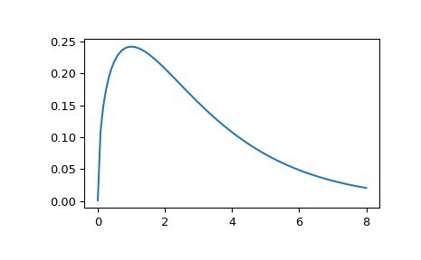
>>> import numpy as np
>>> import matplotlib.pyplot as plt
>>> from scipy.stats import wishart, chi2
>>> x = np.linspace(1e-5, 8, 100)
>>> w = wishart.pdf(x, df=3, scale=1); w[:5]
array([ 0.00126156,  0.10892176,  0.14793434,  0.17400548,  0.1929669 ])
>>> c = chi2.pdf(x, 3); c[:5]
array([ 0.00126156,  0.10892176,  0.14793434,  0.17400548,  0.1929669 ])
>>> plt.plot(x, w)
>>> plt.show()

The input quantiles can be any shape of array, as long as the last axis labels the components.

Alternatively, the object may be called (as a function) to fix the degrees of freedom and scale parameters, returning a “frozen” Wishart random variable:

>>> rv = wishart(df=1, scale=1)
>>> # Frozen object with the same methods but holding the given
>>> # degrees of freedom and scale fixed.

Go BackOpen In Tab