scipy.stats.truncnorm#
- scipy.stats.truncnorm = <scipy.stats._continuous_distns.truncnorm_gen object>[source]#
A truncated normal continuous random variable.
As an instance of the
rv_continuousclass,truncnormobject inherits from it a collection of generic methods (see below for the full list), and completes them with details specific for this particular distribution.Methods
rvs(a, b, loc=0, scale=1, size=1, random_state=None)
Random variates.
pdf(x, a, b, loc=0, scale=1)
Probability density function.
logpdf(x, a, b, loc=0, scale=1)
Log of the probability density function.
cdf(x, a, b, loc=0, scale=1)
Cumulative distribution function.
logcdf(x, a, b, loc=0, scale=1)
Log of the cumulative distribution function.
sf(x, a, b, loc=0, scale=1)
Survival function (also defined as
1 - cdf, but sf is sometimes more accurate).logsf(x, a, b, loc=0, scale=1)
Log of the survival function.
ppf(q, a, b, loc=0, scale=1)
Percent point function (inverse of
cdf— percentiles).isf(q, a, b, loc=0, scale=1)
Inverse survival function (inverse of
sf).moment(order, a, b, loc=0, scale=1)
Non-central moment of the specified order.
stats(a, b, loc=0, scale=1, moments=’mv’)
Mean(‘m’), variance(‘v’), skew(‘s’), and/or kurtosis(‘k’).
entropy(a, b, loc=0, scale=1)
(Differential) entropy of the RV.
fit(data)
Parameter estimates for generic data. See scipy.stats.rv_continuous.fit for detailed documentation of the keyword arguments.
expect(func, args=(a, b), loc=0, scale=1, lb=None, ub=None, conditional=False, **kwds)
Expected value of a function (of one argument) with respect to the distribution.
median(a, b, loc=0, scale=1)
Median of the distribution.
mean(a, b, loc=0, scale=1)
Mean of the distribution.
var(a, b, loc=0, scale=1)
Variance of the distribution.
std(a, b, loc=0, scale=1)
Standard deviation of the distribution.
interval(confidence, a, b, loc=0, scale=1)
Confidence interval with equal areas around the median.
Notes
This distribution is the normal distribution centered on
loc(default 0), with standard deviationscale(default 1), and truncated ataandbstandard deviations fromloc. For arbitrarylocandscale,aandbare not the abscissae at which the shifted and scaled distribution is truncated.Note
If
a_truncandb_truncare the abscissae at which we wish to truncate the distribution (as opposed to the number of standard deviations fromloc), then we can calculate the distribution parametersaandbas follows:a, b = (a_trunc - loc) / scale, (b_trunc - loc) / scale
This is a common point of confusion. For additional clarification, please see the example below.
Examples
>>> import numpy as np
>>> from scipy.stats import truncnorm
>>> import matplotlib.pyplot as plt
>>> fig, ax = plt.subplots(1, 1)
Get the support:
>>> a, b = 0.1, 2
>>> lb, ub = truncnorm.support(a, b)
Calculate the first four moments:
>>> mean, var, skew, kurt = truncnorm.stats(a, b, moments='mvsk')
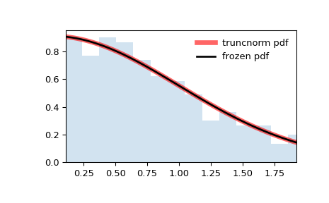
Display the probability density function (
pdf):>>> x = np.linspace(truncnorm.ppf(0.01, a, b), ... truncnorm.ppf(0.99, a, b), 100) >>> ax.plot(x, truncnorm.pdf(x, a, b), ... 'r-', lw=5, alpha=0.6, label='truncnorm pdf')
Alternatively, the distribution object can be called (as a function) to fix the shape, location and scale parameters. This returns a “frozen” RV object holding the given parameters fixed.
Freeze the distribution and display the frozen
pdf:>>> rv = truncnorm(a, b) >>> ax.plot(x, rv.pdf(x), 'k-', lw=2, label='frozen pdf')
Check accuracy of
cdfandppf:>>> vals = truncnorm.ppf([0.001, 0.5, 0.999], a, b) >>> np.allclose([0.001, 0.5, 0.999], truncnorm.cdf(vals, a, b)) True
Generate random numbers:
>>> r = truncnorm.rvs(a, b, size=1000)
And compare the histogram:
>>> ax.hist(r, density=True, bins='auto', histtype='stepfilled', alpha=0.2)
>>> ax.set_xlim([x[0], x[-1]])
>>> ax.legend(loc='best', frameon=False)
>>> plt.show()
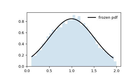
In the examples above,
loc=0andscale=1, so the plot is truncated ataon the left andbon the right. However, suppose we were to produce the same histogram withloc = 1andscale=0.5.>>> loc, scale = 1, 0.5 >>> rv = truncnorm(a, b, loc=loc, scale=scale) >>> x = np.linspace(truncnorm.ppf(0.01, a, b), ... truncnorm.ppf(0.99, a, b), 100) >>> r = rv.rvs(size=1000)
>>> fig, ax = plt.subplots(1, 1)
>>> ax.plot(x, rv.pdf(x), 'k-', lw=2, label='frozen pdf')
>>> ax.hist(r, density=True, bins='auto', histtype='stepfilled', alpha=0.2)
>>> ax.set_xlim(a, b)
>>> ax.legend(loc='best', frameon=False)
>>> plt.show()
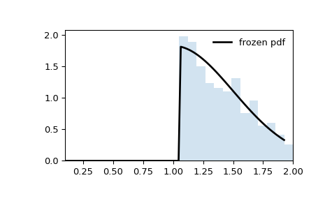
Note that the distribution is no longer appears to be truncated at abscissae
aandb. That is because the standard normal distribution is first truncated ataandb, then the resulting distribution is scaled byscaleand shifted byloc. If we instead want the shifted and scaled distribution to be truncated ataandb, we need to transform these values before passing them as the distribution parameters.>>> a_transformed, b_transformed = (a - loc) / scale, (b - loc) / scale >>> rv = truncnorm(a_transformed, b_transformed, loc=loc, scale=scale) >>> x = np.linspace(truncnorm.ppf(0.01, a, b), ... truncnorm.ppf(0.99, a, b), 100) >>> r = rv.rvs(size=10000)
>>> fig, ax = plt.subplots(1, 1)
>>> ax.plot(x, rv.pdf(x), 'k-', lw=2, label='frozen pdf')
>>> ax.hist(r, density=True, bins='auto', histtype='stepfilled', alpha=0.2)
>>> ax.set_xlim(a-0.1, b+0.1)
>>> ax.legend(loc='best', frameon=False)
>>> plt.show()