scipy.stats.levene#
- scipy.stats.levene(*samples, center='median', proportiontocut=0.05, axis=0, nan_policy='propagate', keepdims=False)[source]#
Perform Levene test for equal variances.
The Levene test tests the null hypothesis that all input samples are from populations with equal variances. Levene’s test is an alternative to Bartlett’s test
bartlettin the case where there are significant deviations from normality.- Parameters:
- sample1, sample2, …array_like
The sample data, possibly with different lengths. Only one-dimensional samples are accepted.
- center{‘mean’, ‘median’, ‘trimmed’}, optional
Which function of the data to use in the test. The default is ‘median’.
- proportiontocutfloat, optional
When center is ‘trimmed’, this gives the proportion of data points to cut from each end. (See
scipy.stats.trim_mean.) Default is 0.05.- axisint or None, default: 0
If an int, the axis of the input along which to compute the statistic. The statistic of each axis-slice (e.g. row) of the input will appear in a corresponding element of the output. If
None, the input will be raveled before computing the statistic.- nan_policy{‘propagate’, ‘omit’, ‘raise’}
Defines how to handle input NaNs.
propagate: if a NaN is present in the axis slice (e.g. row) along which the statistic is computed, the corresponding entry of the output will be NaN.omit: NaNs will be omitted when performing the calculation. If insufficient data remains in the axis slice along which the statistic is computed, the corresponding entry of the output will be NaN.raise: if a NaN is present, aValueErrorwill be raised.
- keepdimsbool, default: False
If this is set to True, the axes which are reduced are left in the result as dimensions with size one. With this option, the result will broadcast correctly against the input array.
- Returns:
- statisticfloat
The test statistic.
- pvaluefloat
The p-value for the test.
See also
Notes
Three variations of Levene’s test are possible. The possibilities and their recommended usages are:
‘median’ : Recommended for skewed (non-normal) distributions>
‘mean’ : Recommended for symmetric, moderate-tailed distributions.
‘trimmed’ : Recommended for heavy-tailed distributions.
The test version using the mean was proposed in the original article of Levene ([2]) while the median and trimmed mean have been studied by Brown and Forsythe ([3]), sometimes also referred to as Brown-Forsythe test.
Beginning in SciPy 1.9,
np.matrixinputs (not recommended for new code) are converted tonp.ndarraybefore the calculation is performed. In this case, the output will be a scalar ornp.ndarrayof appropriate shape rather than a 2Dnp.matrix. Similarly, while masked elements of masked arrays are ignored, the output will be a scalar ornp.ndarrayrather than a masked array withmask=False.References
[2]Levene, H. (1960). In Contributions to Probability and Statistics: Essays in Honor of Harold Hotelling, I. Olkin et al. eds., Stanford University Press, pp. 278-292.
[3]Brown, M. B. and Forsythe, A. B. (1974), Journal of the American Statistical Association, 69, 364-367
[4]C.I. BLISS (1952), The Statistics of Bioassay: With Special Reference to the Vitamins, pp 499-503, DOI:10.1016/C2013-0-12584-6.
[5]B. Phipson and G. K. Smyth. “Permutation P-values Should Never Be Zero: Calculating Exact P-values When Permutations Are Randomly Drawn.” Statistical Applications in Genetics and Molecular Biology 9.1 (2010).
[6]Ludbrook, J., & Dudley, H. (1998). Why permutation tests are superior to t and F tests in biomedical research. The American Statistician, 52(2), 127-132.
Examples
In [4], the influence of vitamin C on the tooth growth of guinea pigs was investigated. In a control study, 60 subjects were divided into small dose, medium dose, and large dose groups that received daily doses of 0.5, 1.0 and 2.0 mg of vitamin C, respectively. After 42 days, the tooth growth was measured.
The
small_dose,medium_dose, andlarge_dosearrays below record tooth growth measurements of the three groups in microns.>>> import numpy as np >>> small_dose = np.array([ ... 4.2, 11.5, 7.3, 5.8, 6.4, 10, 11.2, 11.2, 5.2, 7, ... 15.2, 21.5, 17.6, 9.7, 14.5, 10, 8.2, 9.4, 16.5, 9.7 ... ]) >>> medium_dose = np.array([ ... 16.5, 16.5, 15.2, 17.3, 22.5, 17.3, 13.6, 14.5, 18.8, 15.5, ... 19.7, 23.3, 23.6, 26.4, 20, 25.2, 25.8, 21.2, 14.5, 27.3 ... ]) >>> large_dose = np.array([ ... 23.6, 18.5, 33.9, 25.5, 26.4, 32.5, 26.7, 21.5, 23.3, 29.5, ... 25.5, 26.4, 22.4, 24.5, 24.8, 30.9, 26.4, 27.3, 29.4, 23 ... ])
The
levenestatistic is sensitive to differences in variances between the samples.>>> from scipy import stats >>> res = stats.levene(small_dose, medium_dose, large_dose) >>> res.statistic 0.6457341109631506
The value of the statistic tends to be high when there is a large difference in variances.
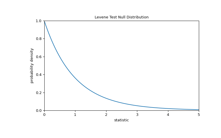
We can test for inequality of variance among the groups by comparing the observed value of the statistic against the null distribution: the distribution of statistic values derived under the null hypothesis that the population variances of the three groups are equal.
For this test, the null distribution follows the F distribution as shown below.
>>> import matplotlib.pyplot as plt
>>> k, n = 3, 60   # number of samples, total number of observations
>>> dist = stats.f(dfn=k-1, dfd=n-k)
>>> val = np.linspace(0, 5, 100)
>>> pdf = dist.pdf(val)
>>> fig, ax = plt.subplots(figsize=(8, 5))
>>> def plot(ax):  # we'll reuse this
...     ax.plot(val, pdf, color='C0')
...     ax.set_title("Levene Test Null Distribution")
...     ax.set_xlabel("statistic")
...     ax.set_ylabel("probability density")
...     ax.set_xlim(0, 5)
...     ax.set_ylim(0, 1)
>>> plot(ax)
>>> plt.show()
The comparison is quantified by the p-value: the proportion of values in the null distribution greater than or equal to the observed value of the statistic.
>>> fig, ax = plt.subplots(figsize=(8, 5))
>>> plot(ax)
>>> pvalue = dist.sf(res.statistic)
>>> annotation = (f'p-value={pvalue:.3f}\n(shaded area)')
>>> props = dict(facecolor='black', width=1, headwidth=5, headlength=8)
>>> _ = ax.annotate(annotation, (1.5, 0.22), (2.25, 0.3), arrowprops=props)
>>> i = val >= res.statistic
>>> ax.fill_between(val[i], y1=0, y2=pdf[i], color='C0')
>>> plt.show()
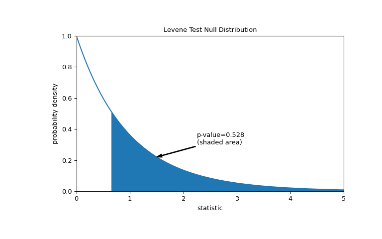
>>> res.pvalue
0.5280694573759905
If the p-value is “small” - that is, if there is a low probability of sampling data from distributions with identical variances that produces such an extreme value of the statistic - this may be taken as evidence against the null hypothesis in favor of the alternative: the variances of the groups are not equal. Note that:
The inverse is not true; that is, the test is not used to provide evidence for the null hypothesis.
The threshold for values that will be considered “small” is a choice that should be made before the data is analyzed [5] with consideration of the risks of both false positives (incorrectly rejecting the null hypothesis) and false negatives (failure to reject a false null hypothesis).
Small p-values are not evidence for a large effect; rather, they can only provide evidence for a “significant” effect, meaning that they are unlikely to have occurred under the null hypothesis.
Note that the F distribution provides an asymptotic approximation of the null distribution. For small samples, it may be more appropriate to perform a permutation test: Under the null hypothesis that all three samples were drawn from the same population, each of the measurements is equally likely to have been observed in any of the three samples. Therefore, we can form a randomized null distribution by calculating the statistic under many randomly-generated partitionings of the observations into the three samples.
>>> def statistic(*samples):
...     return stats.levene(*samples).statistic
>>> ref = stats.permutation_test(
...     (small_dose, medium_dose, large_dose), statistic,
...     permutation_type='independent', alternative='greater'
... )
>>> fig, ax = plt.subplots(figsize=(8, 5))
>>> plot(ax)
>>> bins = np.linspace(0, 5, 25)
>>> ax.hist(
...     ref.null_distribution, bins=bins, density=True, facecolor="C1"
... )
>>> ax.legend(['aymptotic approximation\n(many observations)',
...            'randomized null distribution'])
>>> plot(ax)
>>> plt.show()
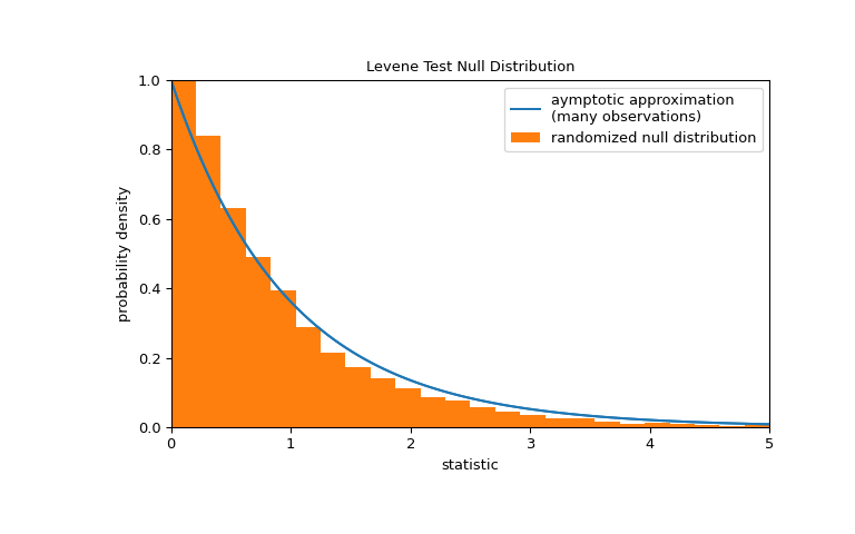
>>> ref.pvalue  # randomized test p-value
0.4559  # may vary
Note that there is significant disagreement between the p-value calculated here and the asymptotic approximation returned by
leveneabove. The statistical inferences that can be drawn rigorously from a permutation test are limited; nonetheless, they may be the preferred approach in many circumstances [6].Following is another generic example where the null hypothesis would be rejected.
Test whether the lists a, b and c come from populations with equal variances.
>>> a = [8.88, 9.12, 9.04, 8.98, 9.00, 9.08, 9.01, 8.85, 9.06, 8.99]
>>> b = [8.88, 8.95, 9.29, 9.44, 9.15, 9.58, 8.36, 9.18, 8.67, 9.05]
>>> c = [8.95, 9.12, 8.95, 8.85, 9.03, 8.84, 9.07, 8.98, 8.86, 8.98]
>>> stat, p = stats.levene(a, b, c)
>>> p
0.002431505967249681
The small p-value suggests that the populations do not have equal variances.
This is not surprising, given that the sample variance of b is much larger than that of a and c:
>>> [np.var(x, ddof=1) for x in [a, b, c]]
[0.007054444444444413, 0.13073888888888888, 0.008890000000000002]