scipy.special.jv#

scipy.special.jv(v, z, out=None) = <ufunc 'jv'>#

Bessel function of the first kind of real order and complex argument.

Parameters:

varray_like: Order (float).
zarray_like: Argument (float or complex).
outndarray, optional: Optional output array for the function values

Returns:

Jscalar or ndarray: Value of the Bessel function, \(J_v(z)\).

See also

jve: \(J_v\) with leading exponential behavior stripped off.
spherical_jn: spherical Bessel functions.
j0: faster version of this function for order 0.
j1: faster version of this function for order 1.

Notes

For positive v values, the computation is carried out using the AMOS [1] zbesj routine, which exploits the connection to the modified Bessel function \(I_v\),

\[ \begin{align}\begin{aligned}J_v(z) = \exp(v\pi\imath/2) I_v(-\imath z)\qquad (\Im z > 0)\\J_v(z) = \exp(-v\pi\imath/2) I_v(\imath z)\qquad (\Im z < 0)\end{aligned}\end{align} \]

For negative v values the formula,

\[J_{-v}(z) = J_v(z) \cos(\pi v) - Y_v(z) \sin(\pi v)\]

is used, where \(Y_v(z)\) is the Bessel function of the second kind, computed using the AMOS routine zbesy. Note that the second term is exactly zero for integer v; to improve accuracy the second term is explicitly omitted for v values such that v = floor(v).

Not to be confused with the spherical Bessel functions (see spherical_jn).

References

[1]

Donald E. Amos, “AMOS, A Portable Package for Bessel Functions of a Complex Argument and Nonnegative Order”, http://netlib.org/amos/

Examples

Evaluate the function of order 0 at one point.

>>> from scipy.special import jv
>>> jv(0, 1.)
0.7651976865579666

Evaluate the function at one point for different orders.

>>> jv(0, 1.), jv(1, 1.), jv(1.5, 1.)
(0.7651976865579666, 0.44005058574493355, 0.24029783912342725)

The evaluation for different orders can be carried out in one call by providing a list or NumPy array as argument for the v parameter:

>>> jv([0, 1, 1.5], 1.)
array([0.76519769, 0.44005059, 0.24029784])

Evaluate the function at several points for order 0 by providing an array for z.

>>> import numpy as np
>>> points = np.array([-2., 0., 3.])
>>> jv(0, points)
array([ 0.22389078,  1.        , -0.26005195])

If z is an array, the order parameter v must be broadcastable to the correct shape if different orders shall be computed in one call. To calculate the orders 0 and 1 for an 1D array:

>>> orders = np.array([[0], [1]])
>>> orders.shape
(2, 1)

>>> jv(orders, points)
array([[ 0.22389078,  1.        , -0.26005195],
       [-0.57672481,  0.        ,  0.33905896]])

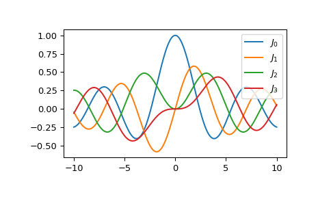
Plot the functions of order 0 to 3 from -10 to 10.

>>> import matplotlib.pyplot as plt
>>> fig, ax = plt.subplots()
>>> x = np.linspace(-10., 10., 1000)
>>> for i in range(4):
...     ax.plot(x, jv(i, x), label=f'$J_{i!r}$')
>>> ax.legend()
>>> plt.show()