scipy.signal.gausspulse#

scipy.signal.gausspulse(t, fc=1000, bw=0.5, bwr=-6, tpr=-60, retquad=False, retenv=False)[source]#

Return a Gaussian modulated sinusoid:

exp(-a t^2) exp(1j*2*pi*fc*t).

If retquad is True, then return the real and imaginary parts (in-phase and quadrature). If retenv is True, then return the envelope (unmodulated signal). Otherwise, return the real part of the modulated sinusoid.

Parameters:

tndarray or the string ‘cutoff’: Input array.
fcfloat, optional: Center frequency (e.g. Hz). Default is 1000.
bwfloat, optional: Fractional bandwidth in frequency domain of pulse (e.g. Hz). Default is 0.5.
bwrfloat, optional: Reference level at which fractional bandwidth is calculated (dB). Default is -6.
tprfloat, optional: If t is ‘cutoff’, then the function returns the cutoff time for when the pulse amplitude falls below tpr (in dB). Default is -60.
retquadbool, optional: If True, return the quadrature (imaginary) as well as the real part of the signal. Default is False.
retenvbool, optional: If True, return the envelope of the signal. Default is False.

Returns:

yIndarray: Real part of signal. Always returned.
yQndarray: Imaginary part of signal. Only returned if retquad is True.
yenvndarray: Envelope of signal. Only returned if retenv is True.

See also

scipy.signal.morlet

Examples

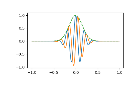
Plot real component, imaginary component, and envelope for a 5 Hz pulse, sampled at 100 Hz for 2 seconds:

>>> import numpy as np
>>> from scipy import signal
>>> import matplotlib.pyplot as plt
>>> t = np.linspace(-1, 1, 2 * 100, endpoint=False)
>>> i, q, e = signal.gausspulse(t, fc=5, retquad=True, retenv=True)
>>> plt.plot(t, i, t, q, t, e, '--')

../../_images/scipy-signal-gausspulse-1.png