Signal Processing (scipy.signal)#
The signal processing toolbox currently contains some filtering functions, a limited set of filter design tools, and a few B-spline interpolation algorithms for 1- and 2-D data. While the B-spline algorithms could technically be placed under the interpolation category, they are included here because they only work with equally-spaced data and make heavy use of filter-theory and transfer-function formalism to provide a fast B-spline transform. To understand this section, you will need to understand that a signal in SciPy is an array of real or complex numbers.
B-splines#
A B-spline is an approximation of a continuous function over a finite- domain in terms of B-spline coefficients and knot points. If the knot- points are equally spaced with spacing \(\Delta x\), then the B-spline approximation to a 1-D function is the finite-basis expansion.
In two dimensions with knot-spacing \(\Delta x\) and \(\Delta y\), the function representation is
In these expressions, \(\beta^{o}\left(\cdot\right)\) is the space-limited B-spline basis function of order \(o\). The requirement of equally-spaced knot-points and equally-spaced data points, allows the development of fast (inverse-filtering) algorithms for determining the coefficients, \(c_{j}\), from sample-values, \(y_{n}\). Unlike the general spline interpolation algorithms, these algorithms can quickly find the spline coefficients for large images.
The advantage of representing a set of samples via B-spline basis functions is that continuous-domain operators (derivatives, re- sampling, integral, etc.), which assume that the data samples are drawn from an underlying continuous function, can be computed with relative ease from the spline coefficients. For example, the second derivative of a spline is
Using the property of B-splines that
it can be seen that
If \(o=3\), then at the sample points:
Thus, the second-derivative signal can be easily calculated from the spline fit. If desired, smoothing splines can be found to make the second derivative less sensitive to random errors.
The savvy reader will have already noticed that the data samples are related to the knot coefficients via a convolution operator, so that simple convolution with the sampled B-spline function recovers the original data from the spline coefficients. The output of convolutions can change depending on how the boundaries are handled (this becomes increasingly more important as the number of dimensions in the dataset increases). The algorithms relating to B-splines in the signal-processing subpackage assume mirror-symmetric boundary conditions. Thus, spline coefficients are computed based on that assumption, and data-samples can be recovered exactly from the spline coefficients by assuming them to be mirror-symmetric also.
Currently the package provides functions for determining second- and third-
order cubic spline coefficients from equally-spaced samples in one and two
dimensions (qspline1d, qspline2d, cspline1d,
cspline2d). For large \(o\), the B-spline basis
function can be approximated well by a zero-mean Gaussian function with
standard-deviation equal to \(\sigma_{o}=\left(o+1\right)/12\) :
A function to compute this Gaussian for arbitrary \(x\) and \(o\) is
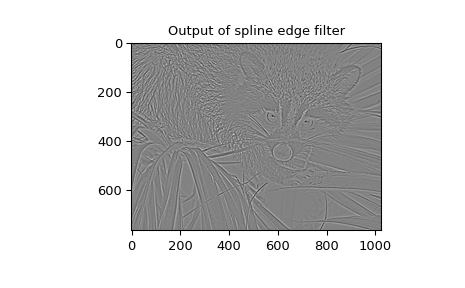
also available ( gauss_spline ). The following code and figure use
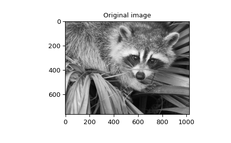
spline-filtering to compute an edge-image (the second derivative of a smoothed
spline) of a raccoon’s face, which is an array returned by the command scipy.datasets.face.
The command sepfir2d was used to apply a separable 2-D FIR
filter with mirror-symmetric boundary conditions to the spline coefficients.
This function is ideally-suited for reconstructing samples from spline
coefficients and is faster than convolve2d, which convolves arbitrary
2-D filters and allows for choosing mirror-symmetric boundary
conditions.
>>> import numpy as np
>>> from scipy import signal, datasets
>>> import matplotlib.pyplot as plt
>>> image = datasets.face(gray=True).astype(np.float32)
>>> derfilt = np.array([1.0, -2, 1.0], dtype=np.float32)
>>> ck = signal.cspline2d(image, 8.0)
>>> deriv = (signal.sepfir2d(ck, derfilt, [1]) +
...          signal.sepfir2d(ck, [1], derfilt))
Alternatively, we could have done:
laplacian = np.array([[0,1,0], [1,-4,1], [0,1,0]], dtype=np.float32)
deriv2 = signal.convolve2d(ck,laplacian,mode='same',boundary='symm')
>>> plt.figure()
>>> plt.imshow(image)
>>> plt.gray()
>>> plt.title('Original image')
>>> plt.show()

>>> plt.figure()
>>> plt.imshow(deriv)
>>> plt.gray()
>>> plt.title('Output of spline edge filter')
>>> plt.show()
Filtering#
Filtering is a generic name for any system that modifies an input signal in some way. In SciPy, a signal can be thought of as a NumPy array. There are different kinds of filters for different kinds of operations. There are two broad kinds of filtering operations: linear and non-linear. Linear filters can always be reduced to multiplication of the flattened NumPy array by an appropriate matrix resulting in another flattened NumPy array. Of course, this is not usually the best way to compute the filter, as the matrices and vectors involved may be huge. For example, filtering a \(512 \times 512\) image with this method would require multiplication of a \(512^2 \times 512^2\) matrix with a \(512^2\) vector. Just trying to store the \(512^2 \times 512^2\) matrix using a standard NumPy array would require \(68,719,476,736\) elements. At 4 bytes per element this would require \(256\textrm{GB}\) of memory. In most applications, most of the elements of this matrix are zero and a different method for computing the output of the filter is employed.
Convolution/Correlation#
Many linear filters also have the property of shift-invariance. This means that the filtering operation is the same at different locations in the signal and it implies that the filtering matrix can be constructed from knowledge of one row (or column) of the matrix alone. In this case, the matrix multiplication can be accomplished using Fourier transforms.
Let \(x\left[n\right]\) define a 1-D signal indexed by the integer \(n.\) Full convolution of two 1-D signals can be expressed as
This equation can only be implemented directly if we limit the sequences to finite-support sequences that can be stored in a computer, choose \(n=0\) to be the starting point of both sequences, let \(K+1\) be that value for which \(x\left[n\right]=0\) for all \(n\geq K+1\) and \(M+1\) be that value for which \(h\left[n\right]=0\) for all \(n\geq M+1\), then the discrete convolution expression is
For convenience, assume \(K\geq M.\) Then, more explicitly, the output of this operation is
Thus, the full discrete convolution of two finite sequences of lengths \(K+1\) and \(M+1\), respectively, results in a finite sequence of length \(K+M+1=\left(K+1\right)+\left(M+1\right)-1.\)
1-D convolution is implemented in SciPy with the function
convolve. This function takes as inputs the signals \(x,\)
\(h\), and two optional flags ‘mode’ and ‘method’, and returns the signal
\(y.\)
The first optional flag, ‘mode’, allows for the specification of which part of the output signal to return. The default value of ‘full’ returns the entire signal. If the flag has a value of ‘same’, then only the middle \(K\) values are returned, starting at \(y\left[\left\lfloor \frac{M-1}{2}\right\rfloor \right]\), so that the output has the same length as the first input. If the flag has a value of ‘valid’, then only the middle \(K-M+1=\left(K+1\right)-\left(M+1\right)+1\) output values are returned, where \(z\) depends on all of the values of the smallest input from \(h\left[0\right]\) to \(h\left[M\right].\) In other words, only the values \(y\left[M\right]\) to \(y\left[K\right]\) inclusive are returned.
The second optional flag, ‘method’, determines how the convolution is computed,
either through the Fourier transform approach with fftconvolve or
through the direct method. By default, it selects the expected faster method.
The Fourier transform method has order \(O(N\log N)\), while the direct
method has order \(O(N^2)\). Depending on the big O constant and the value
of \(N\), one of these two methods may be faster. The default value, ‘auto’,
performs a rough calculation and chooses the expected faster method, while the
values ‘direct’ and ‘fft’ force computation with the other two methods.
The code below shows a simple example for convolution of 2 sequences:
>>> x = np.array([1.0, 2.0, 3.0])
>>> h = np.array([0.0, 1.0, 0.0, 0.0, 0.0])
>>> signal.convolve(x, h)
array([ 0.,  1.,  2.,  3.,  0.,  0.,  0.])
>>> signal.convolve(x, h, 'same')
array([ 2.,  3.,  0.])
This same function convolve can actually take N-D
arrays as inputs and will return the N-D convolution of the
two arrays, as is shown in the code example below. The same input flags are
available for that case as well.
>>> x = np.array([[1., 1., 0., 0.], [1., 1., 0., 0.], [0., 0., 0., 0.], [0., 0., 0., 0.]])
>>> h = np.array([[1., 0., 0., 0.], [0., 0., 0., 0.], [0., 0., 1., 0.], [0., 0., 0., 0.]])
>>> signal.convolve(x, h)
array([[ 1.,  1.,  0.,  0.,  0.,  0.,  0.],
       [ 1.,  1.,  0.,  0.,  0.,  0.,  0.],
       [ 0.,  0.,  1.,  1.,  0.,  0.,  0.],
       [ 0.,  0.,  1.,  1.,  0.,  0.,  0.],
       [ 0.,  0.,  0.,  0.,  0.,  0.,  0.],
       [ 0.,  0.,  0.,  0.,  0.,  0.,  0.],
       [ 0.,  0.,  0.,  0.,  0.,  0.,  0.]])
Correlation is very similar to convolution except that the minus sign becomes a plus sign. Thus,
is the (cross) correlation of the signals \(y\) and \(x.\) For finite-length signals with \(y\left[n\right]=0\) outside of the range \(\left[0,K\right]\) and \(x\left[n\right]=0\) outside of the range \(\left[0,M\right],\) the summation can simplify to
Assuming again that \(K\geq M\), this is
The SciPy function correlate implements this operation. Equivalent
flags are available for this operation to return the full \(K+M+1\) length
sequence (‘full’) or a sequence with the same size as the largest sequence
starting at \(w\left[-K+\left\lfloor \frac{M-1}{2}\right\rfloor \right]\)
(‘same’) or a sequence where the values depend on all the values of the
smallest sequence (‘valid’). This final option returns the \(K-M+1\)
values \(w\left[M-K\right]\) to \(w\left[0\right]\) inclusive.
The function correlate can also take arbitrary N-D arrays as input
and return the N-D convolution of the two arrays on output.
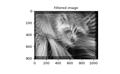
When \(N=2,\) correlate and/or convolve can be used
to construct arbitrary image filters to perform actions such as blurring,
enhancing, and edge-detection for an image.
>>> import numpy as np
>>> from scipy import signal, datasets
>>> import matplotlib.pyplot as plt
>>> image = datasets.face(gray=True)
>>> w = np.zeros((50, 50))
>>> w[0][0] = 1.0
>>> w[49][25] = 1.0
>>> image_new = signal.fftconvolve(image, w)
>>> plt.figure()
>>> plt.imshow(image)
>>> plt.gray()
>>> plt.title('Original image')
>>> plt.show()
>>> plt.figure()
>>> plt.imshow(image_new)
>>> plt.gray()
>>> plt.title('Filtered image')
>>> plt.show()
Calculating the convolution in the time domain as above is mainly used for
filtering when one of the signals is much smaller than the other ( \(K\gg
M\) ), otherwise linear filtering is more efficiently calculated in the
frequency domain provided by the function fftconvolve. By default,
convolve estimates the fastest method using choose_conv_method.
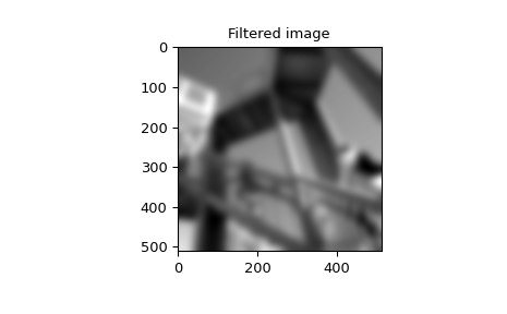
If the filter function \(w[n,m]\) can be factored according to
convolution can be calculated by means of the function sepfir2d. As an
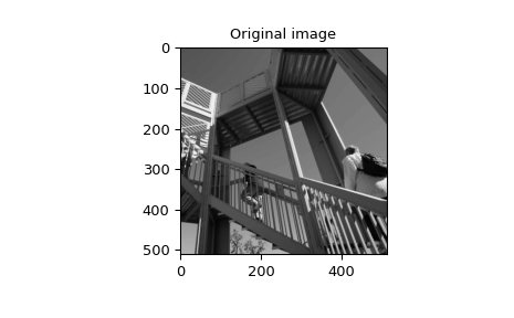
example, we consider a Gaussian filter gaussian
which is often used for blurring.
>>> import numpy as np
>>> from scipy import signal, datasets
>>> import matplotlib.pyplot as plt
>>> image = np.asarray(datasets.ascent(), np.float64)
>>> w = signal.windows.gaussian(51, 10.0)
>>> image_new = signal.sepfir2d(image, w, w)
>>> plt.figure()
>>> plt.imshow(image)
>>> plt.gray()
>>> plt.title('Original image')
>>> plt.show()
>>> plt.figure()
>>> plt.imshow(image_new)
>>> plt.gray()
>>> plt.title('Filtered image')
>>> plt.show()
Difference-equation filtering#
A general class of linear 1-D filters (that includes convolution filters) are filters described by the difference equation
where \(x\left[n\right]\) is the input sequence and \(y\left[n\right]\) is the output sequence. If we assume initial rest so that \(y\left[n\right]=0\) for \(n<0\), then this kind of filter can be implemented using convolution. However, the convolution filter sequence \(h\left[n\right]\) could be infinite if \(a_{k}\neq0\) for \(k\geq1.\) In addition, this general class of linear filter allows initial conditions to be placed on \(y\left[n\right]\) for \(n<0\) resulting in a filter that cannot be expressed using convolution.
The difference equation filter can be thought of as finding \(y\left[n\right]\) recursively in terms of its previous values
Often, \(a_{0}=1\) is chosen for normalization. The implementation in SciPy of this general difference equation filter is a little more complicated than would be implied by the previous equation. It is implemented so that only one signal needs to be delayed. The actual implementation equations are (assuming \(a_{0}=1\) ):
where \(K=\max\left(N,M\right).\) Note that \(b_{K}=0\) if \(K>M\) and \(a_{K}=0\) if \(K>N.\) In this way, the output at time \(n\) depends only on the input at time \(n\) and the value of \(z_{0}\) at the previous time. This can always be calculated as long as the \(K\) values \(z_{0}\left[n-1\right]\ldots z_{K-1}\left[n-1\right]\) are computed and stored at each time step.
The difference-equation filter is called using the command lfilter in
SciPy. This command takes as inputs the vector \(b,\) the vector,
\(a,\) a signal \(x\) and returns the vector \(y\) (the same
length as \(x\) ) computed using the equation given above. If \(x\) is
N-D, then the filter is computed along the axis provided.
If desired, initial conditions providing the values of
\(z_{0}\left[-1\right]\) to \(z_{K-1}\left[-1\right]\) can be provided
or else it will be assumed that they are all zero. If initial conditions are
provided, then the final conditions on the intermediate variables are also
returned. These could be used, for example, to restart the calculation in the
same state.
Sometimes, it is more convenient to express the initial conditions in terms of the signals \(x\left[n\right]\) and \(y\left[n\right].\) In other words, perhaps you have the values of \(x\left[-M\right]\) to \(x\left[-1\right]\) and the values of \(y\left[-N\right]\) to \(y\left[-1\right]\) and would like to determine what values of \(z_{m}\left[-1\right]\) should be delivered as initial conditions to the difference-equation filter. It is not difficult to show that, for \(0\leq m<K,\)
Using this formula, we can find the initial-condition vector
\(z_{0}\left[-1\right]\) to \(z_{K-1}\left[-1\right]\) given initial
conditions on \(y\) (and \(x\) ). The command lfiltic performs
this function.
As an example, consider the following system:
The code calculates the signal \(y[n]\) for a given signal \(x[n]\);
first for initial conditions \(y[-1] = 0\) (default case), then for
\(y[-1] = 2\) by means of lfiltic.
>>> import numpy as np
>>> from scipy import signal
>>> x = np.array([1., 0., 0., 0.])
>>> b = np.array([1.0/2, 1.0/4])
>>> a = np.array([1.0, -1.0/3])
>>> signal.lfilter(b, a, x)
array([0.5, 0.41666667, 0.13888889, 0.0462963])
>>> zi = signal.lfiltic(b, a, y=[2.])
>>> signal.lfilter(b, a, x, zi=zi)
(array([ 1.16666667,  0.63888889,  0.21296296,  0.07098765]), array([0.02366]))
Note that the output signal \(y[n]\) has the same length as the length as the input signal \(x[n]\).
Analysis of Linear Systems#
Linear system described a linear-difference equation can be fully described by the coefficient vectors \(a\) and \(b\) as was done above; an alternative representation is to provide a factor \(k\), \(N_z\) zeros \(z_k\) and \(N_p\) poles \(p_k\), respectively, to describe the system by means of its transfer function \(H(z)\), according to
This alternative representation can be obtained with the scipy function
tf2zpk; the inverse is provided by zpk2tf.
For the above example we have
>>> b = np.array([1.0/2, 1.0/4])
>>> a = np.array([1.0, -1.0/3])
>>> signal.tf2zpk(b, a)
(array([-0.5]), array([ 0.33333333]), 0.5)
i.e., the system has a zero at \(z=-1/2\) and a pole at \(z=1/3\).
The scipy function freqz allows calculation of the frequency response
of a system described by the coefficients \(a_k\) and \(b_k\). See the
help of the freqz function for a comprehensive example.
Filter Design#
Time-discrete filters can be classified into finite response (FIR) filters and infinite response (IIR) filters. FIR filters can provide a linear phase response, whereas IIR filters cannot. SciPy provides functions for designing both types of filters.
FIR Filter#
The function firwin designs filters according to the window method.
Depending on the provided arguments, the function returns different filter
types (e.g., low-pass, band-pass…).
The example below designs a low-pass and a band-stop filter, respectively.
>>> import numpy as np
>>> import scipy.signal as signal
>>> import matplotlib.pyplot as plt
>>> b1 = signal.firwin(40, 0.5)
>>> b2 = signal.firwin(41, [0.3, 0.8])
>>> w1, h1 = signal.freqz(b1)
>>> w2, h2 = signal.freqz(b2)
>>> plt.title('Digital filter frequency response')
>>> plt.plot(w1, 20*np.log10(np.abs(h1)), 'b')
>>> plt.plot(w2, 20*np.log10(np.abs(h2)), 'r')
>>> plt.ylabel('Amplitude Response (dB)')
>>> plt.xlabel('Frequency (rad/sample)')
>>> plt.grid()
>>> plt.show()
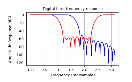
Note that firwin uses, per default, a normalized frequency defined such
that the value \(1\) corresponds to the Nyquist frequency, whereas the
function freqz is defined such that the value \(\pi\) corresponds
to the Nyquist frequency.
The function firwin2 allows design of almost arbitrary frequency
responses by specifying an array of corner frequencies and corresponding
gains, respectively.
The example below designs a filter with such an arbitrary amplitude response.
>>> import numpy as np
>>> import scipy.signal as signal
>>> import matplotlib.pyplot as plt
>>> b = signal.firwin2(150, [0.0, 0.3, 0.6, 1.0], [1.0, 2.0, 0.5, 0.0])
>>> w, h = signal.freqz(b)
>>> plt.title('Digital filter frequency response')
>>> plt.plot(w, np.abs(h))
>>> plt.title('Digital filter frequency response')
>>> plt.ylabel('Amplitude Response')
>>> plt.xlabel('Frequency (rad/sample)')
>>> plt.grid()
>>> plt.show()
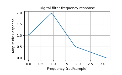
Note the linear scaling of the y-axis and the different definition of the
Nyquist frequency in firwin2 and freqz (as explained above).
IIR Filter#
SciPy provides two functions to directly design IIR iirdesign and
iirfilter, where the filter type (e.g., elliptic) is passed as an
argument and several more filter design functions for specific filter types,
e.g., ellip.
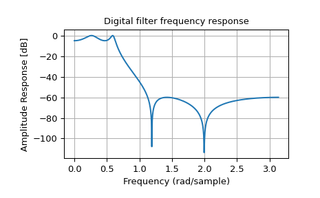
The example below designs an elliptic low-pass filter with defined pass-band and stop-band ripple, respectively. Note the much lower filter order (order 4) compared with the FIR filters from the examples above in order to reach the same stop-band attenuation of \(\approx 60\) dB.
>>> import numpy as np
>>> import scipy.signal as signal
>>> import matplotlib.pyplot as plt
>>> b, a = signal.iirfilter(4, Wn=0.2, rp=5, rs=60, btype='lowpass', ftype='ellip')
>>> w, h = signal.freqz(b, a)
>>> plt.title('Digital filter frequency response')
>>> plt.plot(w, 20*np.log10(np.abs(h)))
>>> plt.title('Digital filter frequency response')
>>> plt.ylabel('Amplitude Response [dB]')
>>> plt.xlabel('Frequency (rad/sample)')
>>> plt.grid()
>>> plt.show()
Filter Coefficients#
Filter coefficients can be stored in several different formats:
‘ba’ or ‘tf’ = transfer function coefficients
‘zpk’ = zeros, poles, and overall gain
‘ss’ = state-space system representation
‘sos’ = transfer function coefficients of second-order sections
Functions, such as tf2zpk and zpk2ss, can convert between them.
Transfer function representation#
The ba or tf format is a 2-tuple (b, a) representing a transfer
function, where b is a length M+1 array of coefficients of the M-order
numerator polynomial, and a is a length N+1 array of coefficients of the
N-order denominator, as positive, descending powers of the transfer function
variable. So the tuple of \(b = [b_0, b_1, ..., b_M]\) and
\(a =[a_0, a_1, ..., a_N]\) can represent an analog filter of the form:
or a discrete-time filter of the form:
This “positive powers” form is found more commonly in controls engineering. If M and N are equal (which is true for all filters generated by the bilinear transform), then this happens to be equivalent to the “negative powers” discrete-time form preferred in DSP:
Although this is true for common filters, remember that this is not true in the general case. If M and N are not equal, the discrete-time transfer function coefficients must first be converted to the “positive powers” form before finding the poles and zeros.
This representation suffers from numerical error at higher orders, so other formats are preferred when possible.
Zeros and poles representation#
The zpk format is a 3-tuple (z, p, k), where z is an M-length
array of the complex zeros of the transfer function
\(z = [z_0, z_1, ..., z_{M-1}]\), p is an N-length array of the
complex poles of the transfer function \(p = [p_0, p_1, ..., p_{N-1}]\),
and k is a scalar gain. These represent the digital transfer function:
or the analog transfer function:
Although the sets of roots are stored as ordered NumPy arrays, their ordering
does not matter: ([-1, -2], [-3, -4], 1) is the same filter as
([-2, -1], [-4, -3], 1).
State-space system representation#
The ss format is a 4-tuple of arrays (A, B, C, D) representing the
state-space of an N-order digital/discrete-time system of the form:
or a continuous/analog system of the form:
with P inputs, Q outputs and N state variables, where:
x is the state vector
y is the output vector of length Q
u is the input vector of length P
A is the state matrix, with shape
(N, N)B is the input matrix with shape
(N, P)C is the output matrix with shape
(Q, N)D is the feedthrough or feedforward matrix with shape
(Q, P). (In cases where the system does not have a direct feedthrough, all values in D are zero.)
State-space is the most general representation and the only one that allows
for multiple-input, multiple-output (MIMO) systems. There are multiple
state-space representations for a given transfer function. Specifically, the
“controllable canonical form” and “observable canonical form” have the same
coefficients as the tf representation, and, therefore, suffer from the same
numerical errors.
Second-order sections representation#
The sos format is a single 2-D array of shape (n_sections, 6),
representing a sequence of second-order transfer functions which, when
cascaded in series, realize a higher-order filter with minimal numerical
error. Each row corresponds to a second-order tf representation, with
the first three columns providing the numerator coefficients and the last
three providing the denominator coefficients:
The coefficients are typically normalized, such that \(a_0\) is always 1. The section order is usually not important with floating-point computation; the filter output will be the same, regardless of the order.
Filter transformations#
The IIR filter design functions first generate a prototype analog low-pass filter with a normalized cutoff frequency of 1 rad/sec. This is then transformed into other frequencies and band types using the following substitutions:
Type |
Transformation |
|---|---|
\(s \rightarrow \frac{s}{\omega_0}\) |
|
\(s \rightarrow \frac{\omega_0}{s}\) |
|
\(s \rightarrow \frac{s^2 + {\omega_0}^2}{s \cdot \mathrm{BW}}\) |
|
\(s \rightarrow \frac{s \cdot \mathrm{BW}}{s^2 + {\omega_0}^2}\) |
Here, \(\omega_0\) is the new cutoff or center frequency, and \(\mathrm{BW}\) is the bandwidth. These preserve symmetry on a logarithmic frequency axis.
To convert the transformed analog filter into a digital filter, the
bilinear transform is used, which makes the following substitution:
where T is the sampling time (the inverse of the sampling frequency).
Other filters#
The signal processing package provides many more filters as well.
Median Filter#
A median filter is commonly applied when noise is markedly non-Gaussian or
when it is desired to preserve edges. The median filter works by sorting all
of the array pixel values in a rectangular region surrounding the point of
interest. The sample median of this list of neighborhood pixel values is used
as the value for the output array. The sample median is the middle-array value
in a sorted list of neighborhood values. If there are an even number of
elements in the neighborhood, then the average of the middle two values is
used as the median. A general purpose median filter that works on
N-D arrays is medfilt. A specialized version that works
only for 2-D arrays is available as medfilt2d.
Order Filter#
A median filter is a specific example of a more general class of filters
called order filters. To compute the output at a particular pixel, all order
filters use the array values in a region surrounding that pixel. These array
values are sorted and then one of them is selected as the output value. For
the median filter, the sample median of the list of array values is used as
the output. A general-order filter allows the user to select which of the
sorted values will be used as the output. So, for example, one could choose to
pick the maximum in the list or the minimum. The order filter takes an
additional argument besides the input array and the region mask that specifies
which of the elements in the sorted list of neighbor array values should be
used as the output. The command to perform an order filter is
order_filter.
Wiener filter#
The Wiener filter is a simple deblurring filter for denoising images. This is not the Wiener filter commonly described in image-reconstruction problems but, instead, it is a simple, local-mean filter. Let \(x\) be the input signal, then the output is
where \(m_{x}\) is the local estimate of the mean and \(\sigma_{x}^{2}\) is the local estimate of the variance. The window for these estimates is an optional input parameter (default is \(3\times3\) ). The parameter \(\sigma^{2}\) is a threshold noise parameter. If \(\sigma\) is not given, then it is estimated as the average of the local variances.
Hilbert filter#
The Hilbert transform constructs the complex-valued analytic signal from a real signal. For example, if \(x=\cos\omega n\), then \(y=\textrm{hilbert}\left(x\right)\) would return (except near the edges) \(y=\exp\left(j\omega n\right).\) In the frequency domain, the hilbert transform performs
where \(H\) is \(2\) for positive frequencies, \(0\) for negative frequencies, and \(1\) for zero-frequencies.
Analog Filter Design#
The functions iirdesign, iirfilter, and the filter design
functions for specific filter types (e.g., ellip) all have a flag
analog, which allows the design of analog filters as well.
The example below designs an analog (IIR) filter, obtains via tf2zpk
the poles and zeros and plots them in the complex s-plane. The zeros at
\(\omega \approx 150\) and \(\omega \approx 300\) can be clearly seen
in the amplitude response.
>>> import numpy as np
>>> import scipy.signal as signal
>>> import matplotlib.pyplot as plt
>>> b, a = signal.iirdesign(wp=100, ws=200, gpass=2.0, gstop=40., analog=True)
>>> w, h = signal.freqs(b, a)
>>> plt.title('Analog filter frequency response')
>>> plt.plot(w, 20*np.log10(np.abs(h)))
>>> plt.ylabel('Amplitude Response [dB]')
>>> plt.xlabel('Frequency')
>>> plt.grid()
>>> plt.show()
!["This code displays two plots. The first plot is an IIR filter response as an X-Y plot with amplitude response on the Y axis vs frequency on the X axis. The low-pass filter shown has a passband from 0 to 100 Hz with 0 dB response and a stop-band from about 175 Hz to 1 KHz about 40 dB down. There are two sharp discontinuities in the filter near 175 Hz and 300 Hz. The second plot is an X-Y showing the transfer function in the complex plane. The Y axis is real-valued an the X axis is complex-valued. The filter has four zeros near [300+0j, 175+0j, -175+0j, -300+0j] shown as blue X markers. The filter also has four poles near [50-30j, -50-30j, 100-8j, -100-8j] shown as red dots."](../_images/signal-7_00_00.png)
>>> z, p, k = signal.tf2zpk(b, a)
>>> plt.plot(np.real(z), np.imag(z), 'ob', markerfacecolor='none')
>>> plt.plot(np.real(p), np.imag(p), 'xr')
>>> plt.legend(['Zeros', 'Poles'], loc=2)
>>> plt.title('Pole / Zero Plot')
>>> plt.xlabel('Real')
>>> plt.ylabel('Imaginary')
>>> plt.grid()
>>> plt.show()
!["This code displays two plots. The first plot is an IIR filter response as an X-Y plot with amplitude response on the Y axis vs frequency on the X axis. The low-pass filter shown has a passband from 0 to 100 Hz with 0 dB response and a stop-band from about 175 Hz to 1 KHz about 40 dB down. There are two sharp discontinuities in the filter near 175 Hz and 300 Hz. The second plot is an X-Y showing the transfer function in the complex plane. The Y axis is real-valued an the X axis is complex-valued. The filter has four zeros near [300+0j, 175+0j, -175+0j, -300+0j] shown as blue X markers. The filter also has four poles near [50-30j, -50-30j, 100-8j, -100-8j] shown as red dots."](../_images/signal-7_01_00.png)
Spectral Analysis#
Spectral analysis refers to investigating the Fourier transform [1] of a signal. Depending on the context, various names, like spectrum, spectral density or periodogram exist for the various spectral representations of the Fourier transform. [2] This section illustrates the most common representations by the example of a continuous-time sine wave signal of fixed duration. Then the use of the discrete Fourier transform [3] on a sampled version of that sine wave is discussed.
Separate subsections are devoted to the spectrum’s phase, estimating the power spectral
density without (periodogram) and with averaging
(welch) as well for non-equally spaced signals
(lombscargle).
Note that the concept of Fourier series is closely related but differs in a crucial point: Fourier series have a spectrum made up of discrete-frequency harmonics, while in this section the spectra are continuous in frequency.
Continuous-time Sine Signal#
Consider a sine signal with amplitude \(a\), frequency \(f_x\) and duration \(\tau\), i.e.,
Since the \(\rect(t)\) function is one for \(|t|<1/2\) and zero for \(|t|>1/2\), it limits \(x(t)\) to the interval \([0, \tau]\). Expressing the sine by complex exponentials shows its two periodic components with frequencies \(\pm f_x\). We assume \(x(t)\) to be a voltage signal, so it has the unit \(\text{V}\).
In signal processing the integral of the absolute square \(|x(t)|^2\) is utilized to define energy and power of a signal, i.e.,
The power \(P_x\) can be interpreted as the energy \(E_x\) per unit time interval. Unit-wise, integrating over \(t\) results in multiplication with seconds. Hence, \(E_x\) has unit \(\text{V}^2\text{s}\) and \(P_x\) has the unit \(\text{V}^2\).
Applying the Fourier transform to \(x(t)\), i.e.,
results in two \(\sinc(f) := \sin(\pi f) /(\pi f)\) functions centered at \(\pm f_x\). The magnitude (absolute value) \(|X(f)|\) has two maxima located at \(\pm f_x\) with value \(|a|\tau/2\). It can be seen in the plot below that \(X(f)\) is not concentrated around the main lobes at \(\pm f_x\), but contains side lobes with heights decreasing proportional to \(1/(\tau f)\). This so-called “spectral leakage” [4] is caused by confining the sine to a finite interval. Note that the shorter the signal duration \(\tau\) is, the higher the leakage. To be independent of the signal duration, the so-called “amplitude spectrum” \(X(f)/\tau\) can be used instead of the spectrum \(X(f)\). Its value at \(f\) corresponds to the amplitude of the complex exponential \(\exp(\jj2\pi f t)\).
Due to Parseval’s theorem, the energy can be calculated from its Fourier transform \(X(f)\) by
as well. E.g., it can be shown by direct calculation that the energy of \(X(f)\) of Eq. (4) is \(|a|^2\tau/2\). Hence, the signal’s power in a frequency band \([f_a, f_b]\) can be determined with
Thus the function \(|X(f)|^2\) can be defined as the so-called “energy spectral density and \(S_{xx}(f) := |X(f)|^2 / \tau\) as “power spectral density” (PSD) of \(x(t)\). Instead of the PSD, the so-called “amplitude spectral density” \(X(f) / \sqrt{\tau}\) is also used, which still contains the phase information. Its absolute square is the PSD and thus it is closely related to the concept of the root-mean-square (RMS) value \(\sqrt{P_x}\) of a signal.
In summary, this subsection presented five ways to represent a spectrum:
Spectrum |
Amplitude Spectrum |
Energy Spectral Density |
Power Spectral Density (PSD) |
Amplitude Spectral Density |
|
|---|---|---|---|---|---|
Definition: |
\(X(f)\) |
\(X(f) / \tau\) |
\(|X(f)|^2\) |
\(|X(f)|^2 / \tau\) |
\(X(f) / \sqrt{\tau}\) |
Magnitude at \(\pm f_x\): |
\(\frac{1}{2}|a|\tau\) |
\(\frac{1}{2}|a|\) |
\(\frac{1}{4}|a|^2\tau^2\) |
\(\frac{1}{4}|a|^2\tau\) |
\(\frac{1}{2}|a|\sqrt{\tau}\) |
Unit: |
\(\text{V} / \text{Hz}\) |
\(\text{V}\) |
\(\text{V}^2\text{s} / \text{Hz}\) |
\(\text{V}^2 / \text{Hz}\) |
\(\text{V} / \sqrt{\text{Hz}}\) |
Note that the units presented in the table above are not unambiguous, e.g., \(\text{V}^2\text{s} / \text{Hz} = \text{V}^2\text{s}^2 = \text{V}^2/ \text{Hz}^2\). When using the absolute value of \(|X(f) / \tau|\) of the amplitude spectrum, it is called a magnitude spectrum. Furthermore, note that the naming scheme of the representations is not consistent and varies in literature.
For real-valued signals the so-called “onesided” spectral representation is often utilized. It only uses the non-negative frequencies (due to \(X(-f)= \conj{X}(f)\) if \(x(t)\in\IR\)). Sometimes the values of the negative frequencies are added to their positive counterparts. Then the amplitude spectrum allows to read off the full (not half) amplitude sine of \(x(t)\) at \(f_z\) and the area of an interval in the PSD represents its full (not half) power. Note that for amplitude spectral densities the positive values are not doubled but multiplied by \(\sqrt{2}\), since it is the square root of the PSD. Furthermore, there is no canonical way for naming a doubled spectrum.
The following plot shows three different spectral representations of four sine signals \(x(t)\) of Eq. (1) with different amplitudes durations \(a\) and durations \(\tau\). For less clutter, the spectra are centered at \(f_z\) and being are plotted next to each other:
import matplotlib.pyplot as plt
import numpy as np

aa = [1, 1, 2, 2]  # amplitudes
taus = [1, 2, 1, 2]  # durations

fg0, axx = plt.subplots(3, 1, sharex='all', tight_layout=True, figsize=(6., 4.))
axx[0].set(title=r"Spectrum $|X(f)|$", ylabel="V/Hz")
axx[1].set(title=r"Magnitude Spectrum $|X(f)/\tau|$ ", ylabel=r"V")
axx[2].set(title=r"Amplitude Spectral Density $|X(f)/\sqrt{\tau}|$",
           ylabel=r"$\operatorname{V} / \sqrt{\operatorname{Hz}}$",
           xlabel="Frequency $f$ in Hertz",)

x_labels, x_ticks = [], []
f = np.linspace(-2.5, 2.5, 400)
for c_, (a_, tau_) in enumerate(zip(aa, taus), start=1):
    aZ_, f_ = abs(a_ * tau_ * np.sinc(tau_ * f) / 2), f + c_ * 5
    axx[0].plot(f_, aZ_)
    axx[1].plot(f_, aZ_ / tau_)
    axx[2].plot(f_, aZ_ / np.sqrt(tau_))
    x_labels.append(rf"$a={a_:g}$, $\tau={tau_:g}$")
    x_ticks.append(c_ * 5)

axx[2].set_xticks(x_ticks)
axx[2].set_xticklabels(x_labels)
plt.show()
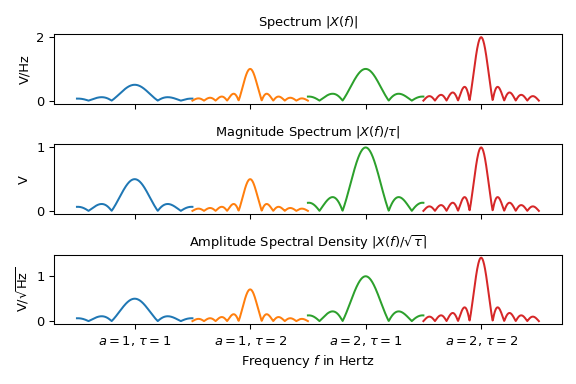
Note that depending on the representation, the height of the peaks vary. Only the interpretation of the magnitude spectrum is straightforward: The peak at \(f_z\) in the second plot represents half the magnitude \(|a|\) of the sine signal. For all other representations the duration \(\tau\) needs to be taken into account to extract information about the signal’s amplitude.
Sampled Sine Signal#
In practice sampled signals are widely used. I.e., the signal is represented by \(n\) samples \(x_k := x(kT)\), \(k=0, \ldots, n-1\), where \(T\) is the sampling interval, \(\tau:=nT\) the signal’s duration and \(f_S := 1/T\) the sampling frequency. Note that the continuous signal needs to be band-limited to \([-f_S/2, f_S/2]\) to avoid aliasing, with \(f_S/2\) being called Nyquist frequency. [5] Replacing the integral by a sum to calculate the signal’s energy and power, i.e.,
delivers the identical result as in the continuous time case of Eq.
(2). The discrete Fourier transform (DFT) and its
inverse (as implemented using efficient FFT calculations in the scipy.fft module)
is given by
The DFT and can be interpreted as an unscaled sampled version of the continuous Fourier transform of Eq. (3), i.e.,
The following plot shows the magnitude spectrum of two sine signals with unit amplitude and frequencies of 20 Hz and 20.5 Hz. The signal is made up of \(n=100\) samples with a sampling interval of \(T=10\) ms resulting in a duration of \(\tau=1\) s and a sampling frequency of \(f_S=100\) Hz.
import matplotlib.pyplot as plt
import numpy as np

from scipy.fft import rfft, rfftfreq

n, T = 100, 0.01  # number of samples and sampling interval
fcc = (20, 20.5)  # frequencies of sines
t = np.arange(n) * T
xx = (np.sin(2 * np.pi * fx_ * t) for fx_ in fcc)  # sine signals

f = rfftfreq(n, T)  # frequency bins range from 0 Hz to Nyquist freq.
XX = (rfft(x_) / n for x_ in xx)  # one-sided magnitude spectrum

fg1, ax1 = plt.subplots(1, 1, tight_layout=True, figsize=(6., 3.))
ax1.set(title=r"Magnitude Spectrum (no window) of $x(t) = \sin(2\pi f_x t)$ ",
        xlabel=rf"Frequency $f$ in Hertz (bin width $\Delta f = {f[1]}\,$Hz)",
        ylabel=r"Magnitude $|X(f)|/\tau$", xlim=(f[0], f[-1]))
for X_, fc_, m_ in zip(XX, fcc, ('x-', '.-')):
    ax1.plot(f, abs(X_), m_, label=rf"$f_x={fc_}\,$Hz")

ax1.grid(True)
ax1.legend()
plt.show()
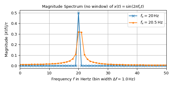
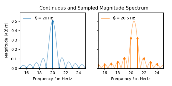
The interpretation of the 20 Hz signal seems straightforward: All values are zero except at 20 Hz. There it is 0.5, which corresponds to half the amplitude of the input signal in accordance with Eq. (1). The peak of the 20.5 Hz signal on the other hand is dispersed along the frequency axis. Eq. (3) shows that this difference is caused by the reason that 20 Hz is a multiple of the bin width of 1 Hz whereas 20.5 Hz is not. The following plot illustrates this by overlaying continuous spectrum over the sampled one:
import matplotlib.pyplot as plt
import numpy as np

from scipy.fft import rfft, rfftfreq

n, T = 100, 0.01  # number of samples and sampling interval
tau = n*T
t = np.arange(n) * T
fcc = (20, 20.5)  # frequencies of sines
xx = (np.sin(2 * np.pi * fc_ * t) for fc_ in fcc)  # sine signals

f = rfftfreq(n, T)  # frequency bins range from 0 Hz to Nyquist freq.
XX = (rfft(x_) / n for x_ in xx)  # one-sided FFT normalized to magnitude

i0, i1 = 15, 25
f_cont = np.linspace(f[i0], f[i1], 501)

fg1, axx = plt.subplots(1, 2, sharey='all', tight_layout=True,
                        figsize=(6., 3.))
for c_, (ax_, X_, fx_) in enumerate(zip(axx, XX, fcc)):
    Xc_ = (np.sinc(tau * (f_cont - fx_)) +
           np.sinc(tau * (f_cont + fx_))) / 2
    ax_.plot(f_cont, abs(Xc_), f'-C{c_}', alpha=.5, label=rf"$f_x={fx_}\,$Hz")
    m_line, _, _, = ax_.stem(f[i0:i1+1], abs(X_[i0:i1+1]), markerfmt=f'dC{c_}',
                             linefmt=f'-C{c_}', basefmt=' ')
    plt.setp(m_line, markersize=5)

    ax_.legend(loc='upper left', frameon=False)
    ax_.set(xlabel="Frequency $f$ in Hertz", xlim=(f[i0], f[i1]),
            ylim=(0, 0.59))

axx[0].set(ylabel=r'Magnitude $|X(f)/\tau|$')
fg1.suptitle("Continuous and Sampled Magnitude Spectrum ", x=0.55, y=0.93)
fg1.tight_layout()
plt.show()
That a slight variation in frequency produces significantly different looking magnitude spectra is obviously undesirable behavior for many practical applications. The following two common techniques can be utilized to improve a spectrum:
The so-called “zero-padding” decreases \(\Delta f\) by appending zeros to the end
of the signal. To oversample the frequency q times, pass the parameter n=q*n_x to
the fft / rfft function with n_x being the
length of the input signal.
The second technique is called windowing, i.e., multiplying the input signal with a suited function such that typically the secondary lobes are suppressed at the cost of widening the main lobe. The windowed DFT can be expressed as
where \(w_k\), \(k=0,\ldots,n-1\) is the sampled window function. To calculate the sampled versions of the spectral representations given in the previous subsection, the following normalization constants
need to be utilized. The first one ensures that a peak in the spectrum is consistent with the signal’s amplitude at that frequency. E.g., the magnitude spectrum can be expressed by \(|X^w_l / c^\text{amp}|\). The second constant guarantees that the power of a frequency interval as defined in Eq. (5) is consistent. The absolute values are needed since complex-valued windows are not forbidden.
The following plot shows the result of applying a hann
window and three times over-sampling to \(x(t)\):
import matplotlib.pyplot as plt
import numpy as np

from scipy.fft import rfft, rfftfreq
from scipy.signal.windows import hann

n, T = 100, 0.01  # number of samples and sampling interval
tau = n*T
q = 3  # over-sampling factor
t = np.arange(n) * T
fcc = (20, 20.5)  # frequencies of sines
xx = [np.sin(2 * np.pi * fc_ * t) for fc_ in fcc]  # sine signals
w = hann(n)
c_w = abs(sum(w))  # normalize constant for window

f_X = rfftfreq(n, T)  # frequency bins range from 0 Hz to Nyquist freq.
XX = (rfft(x_ * w) / c_w for x_ in xx)  # one-sided amplitude spectrum
# Oversampled spectrum:
f_Y = rfftfreq(n*q, T)  # frequency bins range from 0 Hz to Nyquist freq.
YY = (rfft(x_ * w, n=q*n) / c_w for x_ in xx)  # one-sided magnitude spectrum

i0, i1 = 15, 25
j0, j1 = i0*q, i1*q

fg1, axx = plt.subplots(1, 2, sharey='all', tight_layout=True,
                        figsize=(6., 3.))
for c_, (ax_, X_, Y_, fx_) in enumerate(zip(axx, XX, YY, fcc)):
    ax_.plot(f_Y[j0:j1 + 1], abs(Y_[j0:j1 + 1]), f'.-C{c_}',
             label=rf"$f_x={fx_}\,$Hz")
    m_ln, s_ln, _, = ax_.stem(f_X[i0:i1 + 1], abs(X_[i0:i1 + 1]), basefmt=' ',
                              markerfmt=f'dC{c_}', linefmt=f'-C{c_}')
    plt.setp(m_ln, markersize=5)
    plt.setp(s_ln, alpha=0.5)

    ax_.legend(loc='upper left', frameon=False)
    ax_.set(xlabel="Frequency $f$ in Hertz", xlim=(f_X[15], f_X[25]),
            ylim=(0, 0.59))

axx[0].set(ylabel=r'Magnitude $|X(f)/\tau|$')
fg1.suptitle(r"Magnitude Spectrum (Hann window, $%d\times$oversampled)" % q,
             x=0.55, y=0.93)
plt.show()
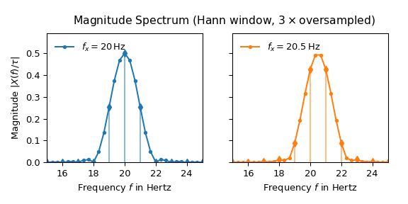
Now both lobes look almost identical and the side lobes are well suppressed. The maximum of the 20.5 Hz spectrum is also very close to the expected height of one half.
Spectral energy and spectral power can be calculated analogously to Eq. (4), yielding in identical results, i.e.,
This formulation is not to be confused with the special case of a rectangular window (or no window), i.e., \(w_k = 1\), \(X^w_l=X_l\), \(c^\text{den}=\sqrt{n}\), which results in
The windowed frequency-discrete power spectral density
is defined over the frequency range \([0, f_S)\) and can be interpreted as power per frequency interval \(\Delta f\). Integrating over a frequency band \([l_a\Delta f, l_b\Delta f)\), like in Eq. (5), becomes the sum
The windowed frequency-discrete energy spectral density \(\tau S^w_{xx}\) can be defined analogously.
The discussion above shows that sampled versions of the spectral representations as in the continuous-time case can be defined. The following tables summarizes these:
Spectrum |
Amplitude Spectrum |
Energy Spectral Density |
Power Spectral Density (PSD) |
Amplitude Spectral Density |
|
|---|---|---|---|---|---|
Definition: |
\(\tau X^w_l / c^\text{amp}\) |
\(X^w_l / c^\text{amp}\) |
\(\tau T |X^w_l / c^\text{den}|^2\) |
\(T |X^w_l / c^\text{den}|^2\) |
\(\sqrt{T} X^w_l / c^\text{den}\) |
Unit: |
\(\text{V} / \text{Hz}\) |
\(\text{V}\) |
\(\text{V}^2\text{s} / \text{Hz}\) |
\(\text{V}^2 / \text{Hz}\) |
\(\text{V} / \sqrt{\text{Hz}}\) |
Note that for the densities, the magnitude values at \(\pm f_x\) differ to the continuous time case due the change from integration to summation for determining spectral energy/power.
Though the hann window is the most common window function used in spectral analysis,
other windows exist. The following plot shows the magnitude spectrum of various window
functions of the windows submodule. It may be interpreted as the
lobe shape of a single frequency input signal. Note that only the right half is shown
and the \(y\)-axis is in decibel, i.e., it is logarithmically scaled.
import matplotlib.pyplot as plt
import numpy as np

from scipy.fft import rfft, rfftfreq
from scipy.signal import get_window

n, n_zp = 128, 16384  # number of samples without and with zero-padding
t = np.arange(n)
f = rfftfreq(n_zp, 1 / n)

ww = ['boxcar', 'hann', 'hamming', 'tukey', 'blackman', 'flattop']
fg0, axx = plt.subplots(len(ww), 1, sharex='all', sharey='all', figsize=(6., 4.))
for c_, (w_name_, ax_) in enumerate(zip(ww, axx)):
    w_ = get_window(w_name_, n, fftbins=False)
    W_ = rfft(w_ / abs(sum(w_)), n=n_zp)
    W_dB = 20*np.log10(np.maximum(abs(W_), 1e-250))
    ax_.plot(f, W_dB, f'C{c_}-', label=w_name_)
    ax_.text(0.1, -50, w_name_, color=f'C{c_}', verticalalignment='bottom',
             horizontalalignment='left', bbox={'color': 'white', 'pad': 0})
    ax_.set_yticks([-20, -60])
    ax_.grid(axis='x')

axx[0].set_title("Spectral Leakage of various Windows")
fg0.supylabel(r"Normalized Magnitude $20\,\log_{10}|W(f)/c^\operatorname{amp}|$ in dB",
              x=0.04, y=0.5, fontsize='medium')
axx[-1].set(xlabel=r"Normalized frequency $f/\Delta f$ in bins",
            xlim=(0, 9), ylim=(-75, 3))

fg0.tight_layout(h_pad=0.4)
plt.show()
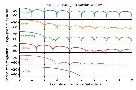
This plot shows that the choice of window function is typically a trade-off between
width of the main lobes and the height of the side lobes. Note that the
boxcar window corresponds to a \(\rect\) function,
i.e., to no windowing. Furthermore, many of the depicted windows are more frequently
used in filter design than in spectral analysis.
Phase of Spectrum#
The phase (i.e., angle) of the Fourier transform is typically utilized
for investigating the time delay of the spectral components of a signal passing through
a system like a filter. In the following example the standard test signal, an impulse
with unit power, is passed through a simple filter, which delays the input by three
samples. The input consists of \(n=50\) samples with sampling interval \(T =
1\) s. The plot shows magnitude and phase over frequency of the input and the output
signal:
import matplotlib.gridspec as gridspec
import matplotlib.pyplot as plt
import numpy as np

from scipy import signal
from scipy.fft import rfft, rfftfreq

# Create input signal:
n = 50
x = np.zeros(n)
x[0] = n

# Apply FIR filter which delays signal by 3 samples:
y = signal.lfilter([0, 0, 0, 1], 1, x)

X, Y = (rfft(z_) / n for z_ in (x, y))
f = rfftfreq(n, 1)  # sampling interval T = 1 s

fig = plt.figure(tight_layout=True, figsize=(6., 4.))
gs = gridspec.GridSpec(3, 1)
ax0 = fig.add_subplot(gs[0, :])
ax1 = fig.add_subplot(gs[1:, :], sharex=ax0)

for Z_, n_, m_ in zip((X, Y), ("Input $X(f)$", "Output $Y(f)$"), ('+-', 'x-')):
    ax0.plot(f, abs(Z_), m_, alpha=.5, label=n_)
    ax1.plot(f, np.unwrap(np.angle(Z_)), m_, alpha=.5, label=n_)

ax0.set(title="Frequency Response of 3 Sample Delay Filter (no window)",
        ylabel="Magnitude", xlim=(0, f[-1]), ylim=(0, 1.1))
ax1.set(xlabel=rf"Frequency $f$ in Hertz ($\Delta f = {1/n}\,$Hz)",
        ylabel=r"Phase in rad")
ax1.set_yticks(-np.arange(0, 7)*np.pi/2,
               ['0', '-π/2', '-π', '-3/2π', '-2π', '-4/3π', '-3π'])

ax2 = ax1.twinx()
ax2.set(ylabel=r"Phase in Degrees", ylim=np.rad2deg(ax1.get_ylim()),
        yticks=np.arange(-540, 90, 90))
for ax_ in (ax0, ax1):
    ax_.legend()
    ax_.grid()
plt.show()
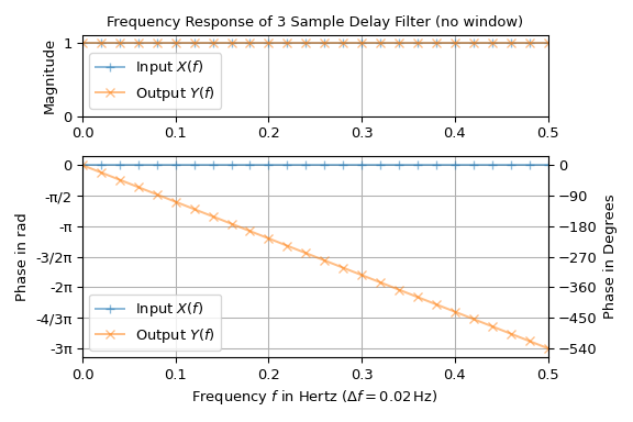
The input has a unit magnitude and zero-phase Fourier transform, which is the reason for the use as a test signal. The output has also unit magnitude but a linearly falling phase with a slope of \(-6\pi\). This is expected, since delaying a signal \(x(t)\) by \(\Delta t\) produces an additional linear phase term in its Fourier transform, i.e.,
Note that in the plot the phase is not limited to the interval \((+\pi, \pi]\)
(output of angle) and hence does not have any discontinuities. This is
achieved by utilizing the numpy.unwrap function. If the transfer function of
the filter is known, freqz can be used to determine the spectral
response of a filter directly.
Spectra with Averaging#
The periodogram function calculates a power spectral density
(scaling='density') or a squared magnitude spectrum (scaling='spectrum'). To
obtain a smoothed periodogram, the welch function can be used. It
does the smoothing by dividing the input signal into overlapping segments, to then
calculate the windowed DFT of each segment. The result is to the average of those DFTs.
The example below shows the squared magnitude spectrum and the power spectral density of a signal made up of a \(1.27\,\text{kHz}\) sine signal with amplitude \(\sqrt{2}\,\text{V}\) and additive gaussian noise having a spectral power density with mean of \(10^{-3}\,\text{V}^2/\text{Hz}\).
import matplotlib.pyplot as plt
import numpy as np
import scipy.signal as signal

rng = np.random.default_rng(73625)  # seeding for reproducibility

fs, n = 10e3, 10_000
f_x, noise_power = 1270, 1e-3 * fs / 2
t = np.arange(n) / fs
x = (np.sqrt(2) * np.sin(2 * np.pi * f_x * t) +
     rng.normal(scale=np.sqrt(noise_power), size=t.shape))

fg, axx = plt.subplots(1, 2, sharex='all', tight_layout=True, figsize=(7, 3.5))
axx[0].set(title="Squared Magnitude Spectrum", ylabel="Square of Magnitude in V²")
axx[1].set(title="Power Spectral Density", ylabel="Power Spectral Density in V²/Hz")
for ax_, s_ in zip(axx, ('spectrum', 'density')):
    f_p, P_p = signal.periodogram(x, fs, 'hann', scaling=s_)
    f_w, P_w = signal.welch(x, fs, scaling=s_)
    ax_.semilogy(f_p/1e3, P_p, label=f"Periodogram ({len(f_p)} bins)")
    ax_.semilogy(f_w/1e3, P_w, label=f"Welch's Method ({len(f_w)} bins)")
    ax_.set(xlabel="Frequency in kHz", xlim=(0, 2), ylim=(1e-7, 1.3))
    ax_.grid(True)
    ax_.legend(loc='lower center')
plt.show()
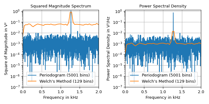
The plots shows that the welch function produces a much smoother
noise floor at the expense of the frequency resolution. Due to the smoothing the height
of sine’s lobe is wider and not as high as in the periodogram. The left plot can be
used to read the height of the lobe, i.e., half sine’s squared magnitude of
\(1\,\text{V}^2\). The right plot can be used to determine the noise floor of
\(10^{-3}\,\text{V}^2/\text{Hz}\). Note that the lobe height of the averaged
squared magnitude spectrum is not exactly one due to limited frequency resolution.
Either zero-padding (e.g., passing nfft=4*len(x) to welch) or
reducing the number of segments by increasing the segment length (setting parameter
nperseg) could be utilized to increase the number of frequency bins.
Lomb-Scargle Periodograms (lombscargle)#
Least-squares spectral analysis (LSSA) [6] [7] is a method of estimating a frequency spectrum, based on a least-squares fit of sinusoids to data samples, similar to Fourier analysis. Fourier analysis, the most used spectral method in science, generally boosts long-periodic noise in long-gapped records; LSSA mitigates such problems.
The Lomb-Scargle method performs spectral analysis on unevenly-sampled data and is known to be a powerful way to find, and test the significance of, weak periodic signals.
For a time series comprising \(N_{t}\) measurements \(X_{j}\equiv X(t_{j})\) sampled at times \(t_{j}\), where \((j = 1, \ldots, N_{t})\), assumed to have been scaled and shifted, such that its mean is zero and its variance is unity, the normalized Lomb-Scargle periodogram at frequency \(f\) is
Here, \(\omega \equiv 2\pi f\) is the angular frequency. The frequency-dependent time offset \(\tau\) is given by
The lombscargle function calculates the periodogram using a slightly
modified algorithm due to Townsend [8], which allows the periodogram to be
calculated using only a single pass through the input arrays for each
frequency.
The equation is refactored as:
and
Here,
while the sums are
This requires \(N_{f}(2N_{t}+3)\) trigonometric function evaluations giving a factor of \(\sim 2\) speed increase over the straightforward implementation.
Short-Time Fourier Transform#
This section gives some background information on using the ShortTimeFFT
class: The short-time Fourier transform (STFT) can be utilized to analyze the
spectral properties of signals over time. It divides a signal into overlapping
chunks by utilizing a sliding window and calculates the Fourier transform
of each chunk. For a continuous-time complex-valued signal \(x(t)\) the
STFT is defined [9] as
where \(w(t)\) is a complex-valued window function with its complex
conjugate being \(\conj{w(t)}\). It can be interpreted as determining the
scalar product of \(x\) with the window \(w\) which is translated by
the time \(t\) and then modulated (i.e., frequency-shifted) by the
frequency \(f\).
For working with sampled signals \(x[k] := x(kT)\), \(k\in\IZ\), with
sampling interval \(T\) (being the inverse of the sampling frequency fs),
the discrete version, i.e., only evaluating the STFT at discrete grid points
\(S[q, p] := S(q \Delta f, p\Delta t)\), \(q,p\in\IZ\), needs to be
used. It can be formulated as
with p representing the time index of \(S\) with time interval
\(\Delta t := h T\), \(h\in\IN\) (see delta_t), which can be
expressed as the hop size of \(h\) samples. \(q\) represents the
frequency index of \(S\) with step size \(\Delta f := 1 / (N T)\)
(see delta_f), which makes it FFT compatible. \(w[m] := w(mT)\),
\(m\in\IZ\) is the sampled window function.
To be more aligned to the implementation of ShortTimeFFT, it makes sense to
reformulate Eq. (7) as a two-step process:
Extract the \(p\)-th slice by windowing with the window \(w[m]\) made up of \(M\) samples (see
m_num) centered at \(t[p] := p \Delta t = h T\) (seedelta_t), i.e.,(8)#\[x_p[m] = x\!\big[m - \lfloor M/2\rfloor + h p\big]\, \conj{w[m]}\ , \quad m = 0, \ldots M-1\ ,\]where the integer \(\lfloor M/2\rfloor\) represents
M//2, i.e, it is the mid point of the window (m_num_mid). For notational convenience, \(x[k]:=0\) for \(k\not\in\{0, 1, \ldots, N-1\}\) is assumed. In the subsection Sliding Windows the indexing of the slices is discussed in more detail.Then perform a discrete Fourier transform (i.e., an FFT) of \(x_p[m]\).
(9)#\[S[q, p] = \sum_{m=0}^{M-1} x_p[m] \exp\!\big\{% -2\jj\pi (q + \phi_m)\, m / M\big\}\ .\]Note that a linear phase \(\phi_m\) (see
phase_shift) can be specified, which corresponds to shifting the input by \(\phi_m\) samples. The default is \(\phi_m = \lfloor M/2\rfloor\) (corresponds per definition tophase_shift = 0), which suppresses linear phase components for unshifted signals. Furthermore, the FFT may be oversampled by padding \(w[m]\) with zeros. This can be achieved by specifyingmfftto be larger than the window lengthm_num—this sets \(M\) tomfft(implying that also \(w[m]:=0\) for \(m\not\in\{0, 1, \ldots, M-1\}\) holds).
The inverse short-time Fourier transform (istft) is implemented by reversing
these two steps:
Perform the inverse discrete Fourier transform, i.e.,
\[x_p[m] = \frac{1}{M}\sum_{q=0}^M S[q, p]\, \exp\!\big\{ 2\jj\pi (q + \phi_m)\, m / M\big\}\ .\]Sum the shifted slices weighted by \(w_d[m]\) to reconstruct the original signal, i.e.,
\[x[k] = \sum_p x_p\!\big[\mu_p(k)\big]\, w_d\!\big[\mu_p(k)\big]\ ,\quad \mu_p(k) = k + \lfloor M/2\rfloor - h p\]for \(k \in [0, \ldots, n-1]\). \(w_d[m]\) is the so-called canonical dual window of \(w[m]\) and is also made up of \(M\) samples.
Note that an inverse STFT does not necessarily exist for all windows and hop sizes. For a given
window \(w[m]\) the hop size \(h\) must be small enough to ensure that
every sample of \(x[k]\) is touched by a non-zero value of at least one
window slice. This is sometimes referred as the “non-zero overlap condition”
(see check_NOLA). Some more details are
given in the subsection Inverse STFT and Dual Windows.
Sliding Windows#
This subsection discusses how the sliding window is indexed in the
ShortTimeFFT by means of an example: Consider a window of length 6 with a
hop interval of two and a sampling interval T of one, e.g., ShortTimeFFT
(np.ones(6), 2, fs=1). The following image schematically depicts the first
four window positions also named time slices:

The x-axis denotes the time \(t\), which corresponds to the sample index
k indicated by the bottom row of blue boxes. The y-axis denotes the time
slice index \(p\). The signal \(x[k]\) starts at index \(k=0\) and
is marked by a light blue background. Per definition the zeroth slice
(\(p=0\)) is centered at \(t=0\). The center of each slice
(m_num_mid), here being the sample 6//2=3, is marked by the text “mid”.
By default the stft calculates all slices which have some overlap with the
signal. Hence the first slice is at p_min = -1 with the lowest sample index
being k_min = -5. The first sample index unaffected by a slice not sticking
out to the left of the signal is \(p_{lb} = 2\) and the first sample index
unaffected by border effects is \(k_{lb} = 5\). The property
lower_border_end returns the tuple \((k_{lb}, p_{lb})\).
The behavior at the end of the signal is depicted for a signal with \(n=50\) samples below, as indicated by the blue background:

Here the last slice has index \(p=26\). Hence, following Python
convention of the end index being outside the range, p_max = 27 indicates the
first slice not touching the signal. The corresponding sample index is
k_max = 55. The first slice, which sticks out to the right is
\(p_{ub} = 24\) with its first sample at \(k_{ub}=45\). The function
upper_border_begin returns the tuple \((k_{ub}, p_{ub})\).
Inverse STFT and Dual Windows#
The term dual window stems from frame theory [10] where a frame is a series expansion which can represent any function in a given Hilbert space. There the expansions \(\{g_k\}\) and \(\{h_k\}\) are dual frames if for all functions \(f\) in the given Hilbert space \(\mathcal{H}\)
holds, where \(\langle ., .\rangle\) denotes the scalar product of \(\mathcal{H}\). All frames have dual frames [10].
An STFT evaluated only at discrete grid
points \(S(q \Delta f, p\Delta t)\) is called a “Gabor frame” in
literature [9] [10].
Since the support of the window \(w[m]\) is limited to a finite interval,
the ShortTimeFFT falls into the class of the so-called “painless
non-orthogonal expansions” [9]. In this case the dual windows always
have the same support and can be calculated by means of inverting a diagonal matrix. A
rough derivation only requiring some understanding of manipulating matrices
will be sketched out in the following:
Since the STFT given in Eq. (7) is a linear mapping in
\(x[k]\), it can be expressed in vector-matrix notation. This allows us to
express the inverse via the formal solution of the linear least squares method
(as in lstsq), which leads to a beautiful and simple result.
We begin by reformulating the windowing of Eq. (8)
where the \(M\times N\) matrix \(\vb{W}_{\!p}\) has only non-zeros entries on the \((ph)\)-th minor diagonal, i.e.,
with \(\delta_{k,l}\) being the Kronecker Delta. Eq. (9) can be expressed as
which allows the STFT of the \(p\)-th slice to be written as
Note that \(\vb{F}\) is unitary, i.e., the inverse equals its conjugate transpose meaning \(\conjT{\vb{F}}\vb{F} = \vb{I}\).
To obtain a single vector-matrix equation for the STFT, the slices are stacked into one vector, i.e.,
where \(P\) is the number of columns of the resulting STFT. To invert this equation the Moore-Penrose inverse \(\vb{G}^\dagger\) can be utilized
which exists if
is invertible. Then \(\vb{x} = \vb{G}^\dagger\vb{G}\,\vb{x} = \inv{\conjT{\vb{G}}\vb{G}}\,\conjT{\vb{G}}\vb{G}\,\vb{x}\) obviously holds. \(\vb{D}\) is always a diagonal matrix with non-negative diagonal entries. This becomes clear, when simplifying \(\vb{D}\) further to
due to \(\vb{F}\) being unitary. Furthermore
shows that \(\vb{D}_p\) is a diagonal matrix with non-negative entries. Hence, summing \(\vb{D}_p\) preserves that property. This allows to simplify Eq. (13) further, i.e,
Utilizing Eq. (11), (14), (15), \(\vb{U}_p=\vb{W}_{\!p}\vb{D}^{-1}\) can be expressed as
This shows \(\vb{U}_p\) has the identical structure as \(\vb{W}_p\) in Eq. (11), i.e., having only non-zero entries on the \((ph)\)-th minor diagonal. The sum term in the inverse can be interpreted as sliding \(|w[\mu]|^2\) over \(w[m]\) (with an incorporated inversion), so only components overlapping with \(w[m]\) have an effect. Hence, all \(U_p[m, k]\) far enough from the border are identical windows. To circumvent border effects, \(x[k]\) is padded with zeros, enlarging \(\vb{U}\) so all slices which touch \(x[k]\) contain the identical dual window
Since \(w[m] = 0\) holds for \(m \not\in\{0, \ldots, M-1\}\), it is only required to sum over the indexes \(\eta\) fulfilling \(|\eta| < M/h\). The name dual window can be justified by inserting Eq. (12) into Eq. (16), i.e.,
showing that \(\vb{U}_p\) and \(\vb{W}_{\!p}\) are interchangeable. Hence, \(w_d[m]\) is also a valid window with dual window \(w[m]\). Note that \(w_d[m]\) is not a unique dual window, due to \(\vb{s}\) typically having more entries than \(\vb{x}\). It can be shown, that \(w_d[m]\) has the minimal energy (or \(L_2\) norm) [9], which is the reason for being named the “canonical dual window”.
Comparison with Legacy Implementation#
The functions stft, istft, and the spectrogram predate the
ShortTimeFFT implementation. This section discusses the key differences
between the older “legacy” and the newer ShortTimeFFT implementations. The
main motivation for a rewrite was the insight that integrating dual
windows could not be done in a sane way without
breaking compatibility. This opened the opportunity for rethinking the code
structure and the parametrization, thus making some implicit behavior more
explicit.
The following example compares the two STFTs of a complex valued chirp signal with a negative slope:
>>> import matplotlib.pyplot as plt
>>> import numpy as np
>>> from scipy.fft import fftshift
>>> from scipy.signal import stft, istft, spectrogram, ShortTimeFFT
...
>>> fs, N = 200, 1001  # 200 Hz sampling rate for 5 s signal
>>> t_z = np.arange(N) / fs  # time indexes for signal
>>> z = np.exp(2j*np.pi*70 * (t_z - 0.2*t_z**2))  # complex-valued chirp
...
>>> nperseg, noverlap = 50, 40
>>> win = ('gaussian', 1e-2 * fs)  # Gaussian with 0.01 s standard dev.
...
>>> # Legacy STFT:
>>> f0_u, t0, Sz0_u = stft(z, fs, win, nperseg, noverlap,
...                        return_onesided=False, scaling='spectrum')
>>> f0, Sz0 = fftshift(f0_u), fftshift(Sz0_u, axes=0)
...
>>> # New STFT:
>>> SFT = ShortTimeFFT.from_window(win, fs, nperseg, noverlap, fft_mode='centered',
...                                scale_to='magnitude', phase_shift=None)
>>> Sz1 = SFT.stft(z)
...
>>> # Plot results:
>>> fig1, axx = plt.subplots(2, 1, sharex='all', sharey='all',
...                          figsize=(6., 5.))  # enlarge figure a bit
>>> t_lo, t_hi, f_lo, f_hi = SFT.extent(N, center_bins=True)
>>> axx[0].set_title(r"Legacy stft() produces $%d\times%d$ points" % Sz0.T.shape)
>>> axx[0].set_xlim(t_lo, t_hi)
>>> axx[0].set_ylim(f_lo, f_hi)
>>> axx[1].set_title(r"ShortTimeFFT produces $%d\times%d$ points" % Sz1.T.shape)
>>> axx[1].set_xlabel(rf"Time $t$ in seconds ($\Delta t= {SFT.delta_t:g}\,$s)")
...
>>> # Calculate extent of plot with centered bins since
>>> # imshow does not interpolate by default:
>>> dt2 = (nperseg-noverlap) / fs / 2  # equals SFT.delta_t / 2
>>> df2 = fs / nperseg / 2  # equals SFT.delta_f / 2
>>> extent0 = (-dt2, t0[-1] + dt2, f0[0] - df2, f0[-1] - df2)
>>> extent1 = SFT.extent(N, center_bins=True)
...
>>> kw = dict(origin='lower', aspect='auto', cmap='viridis')
>>> im1a = axx[0].imshow(abs(Sz0), extent=extent0, **kw)
>>> im1b = axx[1].imshow(abs(Sz1), extent=extent1, **kw)
>>> fig1.colorbar(im1b, ax=axx, label="Magnitude $|S_z(t, f)|$")
>>> _ = fig1.supylabel(r"Frequency $f$ in Hertz ($\Delta f = %g\,$Hz)" %
...                    SFT.delta_f, x=0.08, y=0.5, fontsize='medium')
>>> plt.show()
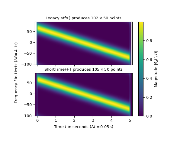
That the ShortTimeFFT produces 3 more time slices than the legacy version is
the main difference. As laid out in the Sliding Windows
section, all slices which touch the signal are incorporated in the new version.
This has the advantage that the STFT can be sliced and reassembled as shown in
the ShortTimeFFT code example. Furthermore, using all touching slices makes
the ISTFT more robust in the case of windows that are zero somewhere.
Note that the slices with identical time stamps produce equal results (up to numerical accuracy), i.e.:
>>> np.allclose(Sz0, Sz1[:, 2:-1])
True
Generally, those additional slices contain non-zero values. Due to the large overlap in our example, they are quite small. E.g.:
>>> abs(Sz1[:, 1]).min(), abs(Sz1[:, 1]).max()
(6.925060911593139e-07, 8.00271269218721e-07)
The ISTFT can be utilized to reconstruct the original signal:
>>> t0_r, z0_r = istft(Sz0_u, fs, win, nperseg, noverlap,
...                    input_onesided=False, scaling='spectrum')
>>> z1_r = SFT.istft(Sz1, k1=N)
...
>>> len(z0_r), len(z)
(1010, 1001)
>>> np.allclose(z0_r[:N], z)
True
>>> np.allclose(z1_r, z)
True
Note that the legacy implementation returns a signal which is longer than the
original. On the other hand, the new istft allows to explicitly specify the
start index k0 and the end index k1 of the reconstructed signal. The length
discrepancy in the old implementation is caused by the fact that the signal
length is not a multiple of the slices.
Further differences between the new and legacy versions in this example are:
The parameter
fft_mode='centered'ensures that the zero frequency is vertically centered for two-sided FFTs in the plot. With the legacy implementation,fftshiftneeds to be utilized.fft_mode='twosided'produces the same behavior as the old version.The parameter
phase_shift=Noneensures identical phases of the two versions.ShortTimeFFT’s default value of0produces STFT slices with an additional linear phase term.
A spectrogram is defined as the absolute square of the STFT [9]. The
spectrogram provided by the ShortTimeFFT sticks to that definition, i.e.:
>>> np.allclose(SFT.spectrogram(z), abs(Sz1)**2)
True
On the other hand, the legacy spectrogram provides another STFT
implementation with the key difference being the different handling of the
signal borders. The following example shows how to use the ShortTimeFFT to
obtain an identical SFT as produced with the legacy spectrogram:
>>> # Legacy spectrogram (detrending for complex signals not useful):
>>> f2_u, t2, Sz2_u = spectrogram(z, fs, win, nperseg, noverlap,
...                               detrend=None, return_onesided=False,
...                               scaling='spectrum', mode='complex')
>>> f2, Sz2 = fftshift(f2_u), fftshift(Sz2_u, axes=0)
...
>>> # New STFT:
... SFT = ShortTimeFFT.from_window(win, fs, nperseg, noverlap,
...                                fft_mode='centered',
...                                scale_to='magnitude', phase_shift=None)
>>> Sz3 = SFT.stft(z, p0=0, p1=(N-noverlap)//SFT.hop, k_offset=nperseg//2)
>>> t3 = SFT.t(N, p0=0, p1=(N-noverlap)//SFT.hop, k_offset=nperseg//2)
...
>>> np.allclose(t2, t3)
True
>>> np.allclose(f2, SFT.f)
True
>>> np.allclose(Sz2, Sz3)
True
The difference from the other STFTs is that the time slices do not start at 0 but
at nperseg//2, i.e.:
>>> t2
array([0.125, 0.175, 0.225, 0.275, 0.325, 0.375, 0.425, 0.475, 0.525,
       ...
       4.625, 4.675, 4.725, 4.775, 4.825, 4.875])
Furthermore, only slices which do not stick out to the right are returned,
centering the last slice at 4.875 s, which makes it shorter than with the default
stft parametrization.
Using the mode parameter, the legacy spectrogram can also return the
‘angle’, ‘phase’, ‘psd’ or the ‘magnitude’. The scaling behavior of the
legacy spectrogram is not straightforward, since it depends on the
parameters mode, scaling and return_onesided. There is no direct
correspondence for all combinations in the ShortTimeFFT, since it provides
only ‘magnitude’, ‘psd’ or no scaling of the window at all. The following
table shows those correspondences:
Legacy |
|||||
|---|---|---|---|---|---|
mode |
scaling |
return_onesided |
|||
psd |
density |
True |
onesided2X |
psd |
|
psd |
density |
False |
twosided |
psd |
|
magnitude |
spectrum |
True |
onesided |
magnitude |
|
magnitude |
spectrum |
False |
twosided |
magnitude |
|
complex |
spectrum |
True |
onesided |
magnitude |
|
complex |
spectrum |
False |
twosided |
magnitude |
|
psd |
spectrum |
True |
— |
— |
|
psd |
spectrum |
False |
— |
— |
|
complex |
density |
True |
— |
— |
|
complex |
density |
False |
— |
— |
|
magnitude |
density |
True |
— |
— |
|
magnitude |
density |
False |
— |
— |
|
— |
— |
— |
|
|
|
When using onesided output on complex-valued input signals, the old
spectrogram switches to two-sided mode. The ShortTimeFFT raises
a TypeError, since the utilized rfft function only accepts
real-valued inputs. Consult the Spectral Analysis section above for a
discussion on the various spectral representations which are induced by the various
parameterizations.
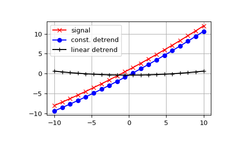
Detrend#
SciPy provides the function detrend to remove a constant or linear
trend in a data series in order to see effect of higher order.
The example below removes the constant and linear trend of a second-order polynomial time series and plots the remaining signal components.
>>> import numpy as np
>>> import scipy.signal as signal
>>> import matplotlib.pyplot as plt
>>> t = np.linspace(-10, 10, 20)
>>> y = 1 + t + 0.01*t**2
>>> yconst = signal.detrend(y, type='constant')
>>> ylin = signal.detrend(y, type='linear')
>>> plt.plot(t, y, '-rx')
>>> plt.plot(t, yconst, '-bo')
>>> plt.plot(t, ylin, '-k+')
>>> plt.grid()
>>> plt.legend(['signal', 'const. detrend', 'linear detrend'])
>>> plt.show()
References
Some further reading and related software: