Optimization (optimize)
There are several classical optimization algorithms provided by SciPy in the scipy.optimize package. An overview of the module is available using help (or pydoc.help):
from scipy import optimize
>>> info(optimize)
Optimization Tools
==================

 A collection of general-purpose optimization routines.

   fmin        --  Nelder-Mead Simplex algorithm
                     (uses only function calls)
   fmin_powell --  Powell's (modified) level set method (uses only
                     function calls)
   fmin_cg     --  Non-linear (Polak-Ribiere) conjugate gradient algorithm
                     (can use function and gradient).
   fmin_bfgs   --  Quasi-Newton method (Broydon-Fletcher-Goldfarb-Shanno);
                     (can use function and gradient)
   fmin_ncg    --  Line-search Newton Conjugate Gradient (can use
                     function, gradient and Hessian).
   leastsq     --  Minimize the sum of squares of M equations in
                     N unknowns given a starting estimate.


  Constrained Optimizers (multivariate)

   fmin_l_bfgs_b -- Zhu, Byrd, and Nocedal's L-BFGS-B constrained optimizer
                      (if you use this please quote their papers -- see help)

   fmin_tnc      -- Truncated Newton Code originally written by Stephen Nash and
                      adapted to C by Jean-Sebastien Roy.

   fmin_cobyla   -- Constrained Optimization BY Linear Approximation


  Global Optimizers

   anneal      --  Simulated Annealing
   brute       --  Brute force searching optimizer


  Scalar function minimizers

   fminbound   --  Bounded minimization of a scalar function.
   brent       --  1-D function minimization using Brent method.
   golden      --  1-D function minimization using Golden Section method
   bracket     --  Bracket a minimum (given two starting points)


 Also a collection of general-purpose root-finding routines.

   fsolve      --  Non-linear multi-variable equation solver.


  Scalar function solvers

   brentq      --  quadratic interpolation Brent method
   brenth      --  Brent method (modified by Harris with hyperbolic
                     extrapolation)
   ridder      --  Ridder's method
   bisect      --  Bisection method
   newton      --  Secant method or Newton's method

   fixed_point --  Single-variable fixed-point solver.

 A collection of general-purpose nonlinear multidimensional solvers.

   broyden1            --  Broyden's first method - is a quasi-Newton-Raphson
                           method for updating an approximate Jacobian and then
                           inverting it
   broyden2            --  Broyden's second method - the same as broyden1, but
                           updates the inverse Jacobian directly
   broyden3            --  Broyden's second method - the same as broyden2, but
                           instead of directly computing the inverse Jacobian,
                           it remembers how to construct it using vectors, and
                           when computing inv(J)*F, it uses those vectors to
                           compute this product, thus avoding the expensive NxN
                           matrix multiplication.
   broyden_generalized --  Generalized Broyden's method, the same as broyden2,
                           but instead of approximating the full NxN Jacobian,
                           it construct it at every iteration in a way that
                           avoids the NxN matrix multiplication.  This is not
                           as precise as broyden3.
   anderson            --  extended Anderson method, the same as the
                           broyden_generalized, but added w_0^2*I to before
                           taking inversion to improve the stability
   anderson2           --  the Anderson method, the same as anderson, but
                           formulated differently

 Utility Functions

   line_search --  Return a step that satisfies the strong Wolfe conditions.
   check_grad  --  Check the supplied derivative using finite difference
                     techniques.
The first four algorithms are unconstrained minimization algorithms (fmin: Nelder-Mead simplex, fmin_bfgs: BFGS, fmin_ncg: Newton Conjugate Gradient, and leastsq: Levenburg-Marquardt). The last algorithm actually finds the roots of a general function of possibly many variables. It is included in the optimization package because at the (non-boundary) extreme points of a function, the gradient is equal to zero.
Nelder-Mead Simplex algorithm (fmin)
The simplex algorithm is probably the simplest way to minimize a
fairly well-behaved function. The simplex algorithm requires only
function evaluations and is a good choice for simple minimization
problems. However, because it does not use any gradient evaluations,
it may take longer to find the minimum. To demonstrate the
minimization function consider the problem of minimizing the
Rosenbrock function of  variables:
![\[ f\left(\mathbf{x}\right)=\sum_{i=1}^{N-1}100\left(x_{i}-x_{i-1}^{2}\right)^{2}+\left(1-x_{i-1}\right)^{2}.\]](../_images/math/2cd91295e06479e61445b54e23852a2e50b14e3c.png)
The minimum value of this function is 0 which is achieved when  This minimum can be found using the fmin routine as shown in the example below:
>>> from scipy.optimize import fmin
>>> def rosen(x):
...     """The Rosenbrock function"""
...     return sum(100.0*(x[1:]-x[:-1]**2.0)**2.0 + (1-x[:-1])**2.0)
>>> x0 = [1.3, 0.7, 0.8, 1.9, 1.2] >>> xopt = fmin(rosen, x0, xtol=1e-8) Optimization terminated successfully. Current function value: 0.000000 Iterations: 339 Function evaluations: 571>>> print xopt [ 1. 1. 1. 1. 1.]
Another optimization algorithm that needs only function calls to find the minimum is Powell’s method available as fmin_powell.
Broyden-Fletcher-Goldfarb-Shanno algorithm (fmin_bfgs)
In order to converge more quickly to the solution, this routine uses the gradient of the objective function. If the gradient is not given by the user, then it is estimated using first-differences. The Broyden-Fletcher-Goldfarb-Shanno (BFGS) method typically requires fewer function calls than the simplex algorithm even when the gradient must be estimated.
To demonstrate this algorithm, the Rosenbrock function is again used. The gradient of the Rosenbrock function is the vector:
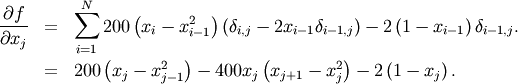
This expression is valid for the interior derivatives. Special cases are
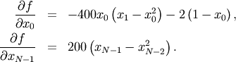
A Python function which computes this gradient is constructed by the code-segment:
>>> def rosen_der(x):
...     xm = x[1:-1]
...     xm_m1 = x[:-2]
...     xm_p1 = x[2:]
...     der = zeros_like(x)
...     der[1:-1] = 200*(xm-xm_m1**2) - 400*(xm_p1 - xm**2)*xm - 2*(1-xm)
...     der[0] = -400*x[0]*(x[1]-x[0]**2) - 2*(1-x[0])
...     der[-1] = 200*(x[-1]-x[-2]**2)
...     return der
The calling signature for the BFGS minimization algorithm is similar to fmin with the addition of the fprime argument. An example usage of fmin_bfgs is shown in the following example which minimizes the Rosenbrock function.
>>> from scipy.optimize import fmin_bfgs>>> x0 = [1.3, 0.7, 0.8, 1.9, 1.2] >>> xopt = fmin_bfgs(rosen, x0, fprime=rosen_der) Optimization terminated successfully. Current function value: 0.000000 Iterations: 53 Function evaluations: 65 Gradient evaluations: 65 >>> print xopt [ 1. 1. 1. 1. 1.]
Newton-Conjugate-Gradient (fmin_ncg)
The method which requires the fewest function calls and is therefore often the fastest method to minimize functions of many variables is fmin_ncg. This method is a modified Newton’s method and uses a conjugate gradient algorithm to (approximately) invert the local Hessian. Newton’s method is based on fitting the function locally to a quadratic form:
![\[ f\left(\mathbf{x}\right)\approx f\left(\mathbf{x}_{0}\right)+\nabla f\left(\mathbf{x}_{0}\right)\cdot\left(\mathbf{x}-\mathbf{x}_{0}\right)+\frac{1}{2}\left(\mathbf{x}-\mathbf{x}_{0}\right)^{T}\mathbf{H}\left(\mathbf{x}_{0}\right)\left(\mathbf{x}-\mathbf{x}_{0}\right).\]](../_images/math/f0534e9ffda6595b8a080dd62dc91952c41ff681.png)
where  is a matrix of second-derivatives (the Hessian). If the Hessian is
positive definite then the local minimum of this function can be found
by setting the gradient of the quadratic form to zero, resulting in
is a matrix of second-derivatives (the Hessian). If the Hessian is
positive definite then the local minimum of this function can be found
by setting the gradient of the quadratic form to zero, resulting in
![\[ \mathbf{x}_{\textrm{opt}}=\mathbf{x}_{0}-\mathbf{H}^{-1}\nabla f.\]](../_images/math/749539f9cd9c8fa6ee61e67cff898b54f3077a5e.png)
The inverse of the Hessian is evaluted using the conjugate-gradient method. An example of employing this method to minimizing the Rosenbrock function is given below. To take full advantage of the NewtonCG method, a function which computes the Hessian must be provided. The Hessian matrix itself does not need to be constructed, only a vector which is the product of the Hessian with an arbitrary vector needs to be available to the minimization routine. As a result, the user can provide either a function to compute the Hessian matrix, or a function to compute the product of the Hessian with an arbitrary vector.
Full Hessian example:
The Hessian of the Rosenbrock function is
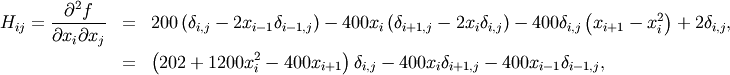
if ![i,j\in\left[1,N-2\right]](../_images/math/a42ca4fb62cec850a850efeec2effe6f60244af0.png) with
with ![i,j\in\left[0,N-1\right]](../_images/math/b0c94de6425aea4ecd9ceb9bea133f399367b9b9.png) defining the
defining the  matrix. Other non-zero entries of the matrix are
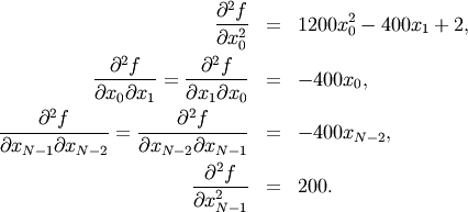
For example, the Hessian when  is
is
![\[ \mathbf{H}=\left[\begin{array}{ccccc} 1200x_{0}^{2}-400x_{1}+2 & -400x_{0} & 0 & 0 & 0\\ -400x_{0} & 202+1200x_{1}^{2}-400x_{2} & -400x_{1} & 0 & 0\\ 0 & -400x_{1} & 202+1200x_{2}^{2}-400x_{3} & -400x_{2} & 0\\ 0 & & -400x_{2} & 202+1200x_{3}^{2}-400x_{4} & -400x_{3}\\ 0 & 0 & 0 & -400x_{3} & 200\end{array}\right].\]](../_images/math/1ca36bb25b64ff242a87c1bc7469fabdbad74271.png)
The code which computes this Hessian along with the code to minimize the function using fmin_ncg is shown in the following example:
>>> from scipy.optimize import fmin_ncg
>>> def rosen_hess(x):
...     x = asarray(x)
...     H = diag(-400*x[:-1],1) - diag(400*x[:-1],-1)
...     diagonal = zeros_like(x)
...     diagonal[0] = 1200*x[0]-400*x[1]+2
...     diagonal[-1] = 200
...     diagonal[1:-1] = 202 + 1200*x[1:-1]**2 - 400*x[2:]
...     H = H + diag(diagonal)
...     return H
>>> x0 = [1.3, 0.7, 0.8, 1.9, 1.2] >>> xopt = fmin_ncg(rosen, x0, rosen_der, fhess=rosen_hess, avextol=1e-8) Optimization terminated successfully. Current function value: 0.000000 Iterations: 23 Function evaluations: 26 Gradient evaluations: 23 Hessian evaluations: 23 >>> print xopt [ 1. 1. 1. 1. 1.]
Hessian product example:
For larger minimization problems, storing the entire Hessian matrix can consume considerable time and memory. The Newton-CG algorithm only needs the product of the Hessian times an arbitrary vector. As a result, the user can supply code to compute this product rather than the full Hessian by setting the fhess_p keyword to the desired function. The fhess_p function should take the minimization vector as the first argument and the arbitrary vector as the second argument. Any extra arguments passed to the function to be minimized will also be passed to this function. If possible, using Newton-CG with the hessian product option is probably the fastest way to minimize the function.
In this case, the product of the Rosenbrock Hessian with an arbitrary
vector is not difficult to compute. If  is the arbitrary vector, then
  has elements:
![\[ \mathbf{H}\left(\mathbf{x}\right)\mathbf{p}=\left[\begin{array}{c} \left(1200x_{0}^{2}-400x_{1}+2\right)p_{0}-400x_{0}p_{1}\\ \vdots\\ -400x_{i-1}p_{i-1}+\left(202+1200x_{i}^{2}-400x_{i+1}\right)p_{i}-400x_{i}p_{i+1}\\ \vdots\\ -400x_{N-2}p_{N-2}+200p_{N-1}\end{array}\right].\]](../_images/math/6c4675fa762e45e8c7b9a55255c3e520ea5d0477.png)
Code which makes use of the fhess_p keyword to minimize the Rosenbrock function using fmin_ncg follows:
>>> from scipy.optimize import fmin_ncg
>>> def rosen_hess_p(x,p):
...     x = asarray(x)
...     Hp = zeros_like(x)
...     Hp[0] = (1200*x[0]**2 - 400*x[1] + 2)*p[0] - 400*x[0]*p[1]
...     Hp[1:-1] = -400*x[:-2]*p[:-2]+(202+1200*x[1:-1]**2-400*x[2:])*p[1:-1] \
...                -400*x[1:-1]*p[2:]
...     Hp[-1] = -400*x[-2]*p[-2] + 200*p[-1]
...     return Hp
>>> x0 = [1.3, 0.7, 0.8, 1.9, 1.2] >>> xopt = fmin_ncg(rosen, x0, rosen_der, fhess_p=rosen_hess_p, avextol=1e-8) Optimization terminated successfully. Current function value: 0.000000 Iterations: 22 Function evaluations: 25 Gradient evaluations: 22 Hessian evaluations: 54 >>> print xopt [ 1. 1. 1. 1. 1.]
Least-square fitting (leastsq)
All of the previously-explained minimization procedures can be used to
solve a least-squares problem provided the appropriate objective
function is constructed. For example, suppose it is desired to fit a
set of data  to a known model,
 where is a vector of parameters for the model that
need to be found. A common method for determining which parameter
vector gives the best fit to the data is to minimize the sum of squares
of the residuals. The residual is usually defined for each observed
data-point as
where is a vector of parameters for the model that
need to be found. A common method for determining which parameter
vector gives the best fit to the data is to minimize the sum of squares
of the residuals. The residual is usually defined for each observed
data-point as
![\[ e_{i}\left(\mathbf{p},\mathbf{y}_{i},\mathbf{x}_{i}\right)=\left\Vert \mathbf{y}_{i}-\mathbf{f}\left(\mathbf{x}_{i},\mathbf{p}\right)\right\Vert .\]](../_images/math/eb3564391ae7831326315a47605a9af7f5e84ba6.png)
An objective function to pass to any of the previous minization algorithms to obtain a least-squares fit is.
![\[ J\left(\mathbf{p}\right)=\sum_{i=0}^{N-1}e_{i}^{2}\left(\mathbf{p}\right).\]](../_images/math/e5d19e9d6d1b9a59962a43d0a22b9a43f45c3b22.png)
The leastsq algorithm performs this squaring and summing of the
residuals automatically. It takes as an input argument the vector
function  and returns the
value of which minimizes
and returns the
value of which minimizes
 directly. The user is also encouraged to provide the Jacobian matrix
of the function (with derivatives down the columns or across the
rows). If the Jacobian is not provided, it is estimated.
directly. The user is also encouraged to provide the Jacobian matrix
of the function (with derivatives down the columns or across the
rows). If the Jacobian is not provided, it is estimated.
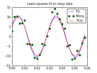
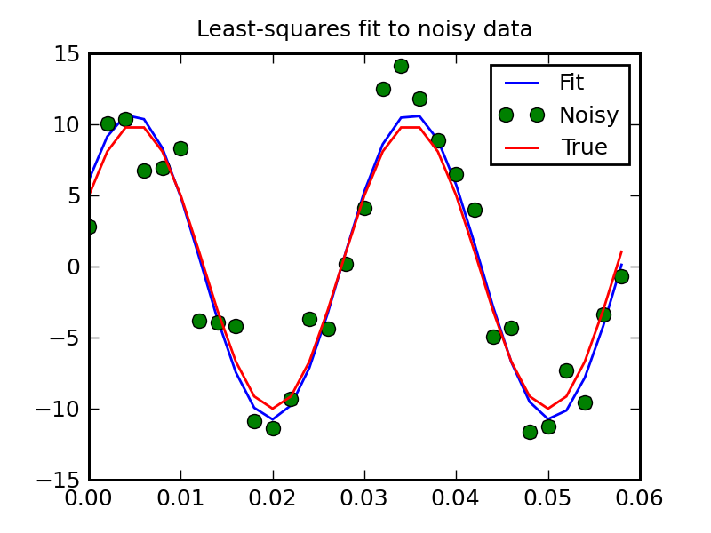
An example should clarify the usage. Suppose it is believed some measured data follow a sinusoidal pattern
![\[ y_{i}=A\sin\left(2\pi kx_{i}+\theta\right)\]](../_images/math/b40b588f31a90a9d06f7e32624641c5d648e4bb9.png)
where the parameters 
 , and
, and  are unknown. The residual vector is
![\[ e_{i}=\left|y_{i}-A\sin\left(2\pi kx_{i}+\theta\right)\right|.\]](../_images/math/e5f48d5aa4cadf0bc8181cf9381276494979d5dc.png)
By defining a function to compute the residuals and (selecting an
appropriate starting position), the least-squares fit routine can be
used to find the best-fit parameters  .
This is shown in the following example:
.
This is shown in the following example:
>>> from numpy import *
>>> x = arange(0,6e-2,6e-2/30)
>>> A,k,theta = 10, 1.0/3e-2, pi/6
>>> y_true = A*sin(2*pi*k*x+theta)
>>> y_meas = y_true + 2*random.randn(len(x))
>>> def residuals(p, y, x): ... A,k,theta = p ... err = y-A*sin(2*pi*k*x+theta) ... return err>>> def peval(x, p): ... return p[0]*sin(2*pi*p[1]*x+p[2])>>> p0 = [8, 1/2.3e-2, pi/3] >>> print array(p0) [ 8. 43.4783 1.0472]>>> from scipy.optimize import leastsq >>> plsq = leastsq(residuals, p0, args=(y_meas, x)) >>> print plsq[0] [ 10.9437 33.3605 0.5834]>>> print array([A, k, theta]) [ 10. 33.3333 0.5236]>>> import matplotlib.pyplot as plt >>> plt.plot(x,peval(x,plsq[0]),x,y_meas,'o',x,y_true) >>> plt.title('Least-squares fit to noisy data') >>> plt.legend(['Fit', 'Noisy', 'True']) >>> plt.show()
(Source code)
Scalar function minimizers
Often only the minimum of a scalar function is needed (a scalar function is one that takes a scalar as input and returns a scalar output). In these circumstances, other optimization techniques have been developed that can work faster.
Unconstrained minimization (brent)
There are actually two methods that can be used to minimize a scalar
function (brent and golden), but golden is
included only for academic purposes and should rarely be used. The
brent method uses Brent’s algorithm for locating a minimum. Optimally
a bracket should be given which contains the minimum desired. A
bracket is a triple  such that
 and
and
 . If this is not given, then alternatively two starting
points can be chosen and a bracket will be found from these points
using a simple marching algorithm. If these two starting points are
not provided 0 and 1 will be used (this may not be the right choice
for your function and result in an unexpected minimum being returned).
. If this is not given, then alternatively two starting
points can be chosen and a bracket will be found from these points
using a simple marching algorithm. If these two starting points are
not provided 0 and 1 will be used (this may not be the right choice
for your function and result in an unexpected minimum being returned).
Bounded minimization (fminbound)
Thus far all of the minimization routines described have been unconstrained minimization routines. Very often, however, there are constraints that can be placed on the solution space before minimization occurs. The fminbound function is an example of a constrained minimization procedure that provides a rudimentary interval constraint for scalar functions. The interval constraint allows the minimization to occur only between two fixed endpoints.
For example, to find the minimum of  near
near  , fminbound can be called using the interval
 ![\left[4,7\right]](../_images/math/fb3f8cdf1cd70a262c58ad6a68d660a3ebdf0017.png) as a constraint. The result is
as a constraint. The result is  :
:
>>> from scipy.special import j1
>>> from scipy.optimize import fminbound
>>> xmin = fminbound(j1, 4, 7)
>>> print xmin
5.33144184241
Root finding
Sets of equations
To find the roots of a polynomial, the command roots is useful. To find a root of a set of non-linear equations, the command fsolve is needed. For example, the following example finds the roots of the single-variable transcendental equation
![\[ x+2\cos\left(x\right)=0,\]](../_images/math/7f83e112da2ff7a423f7ffcd84d834c55a699237.png)
and the set of non-linear equations
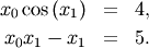
The results are  and
and  .
.
>>> def func(x):
...     return x + 2*cos(x)
>>> def func2(x): ... out = [x[0]*cos(x[1]) - 4] ... out.append(x[1]*x[0] - x[1] - 5) ... return out>>> from scipy.optimize import fsolve >>> x0 = fsolve(func, 0.3) >>> print x0 -1.02986652932>>> x02 = fsolve(func2, [1, 1]) >>> print x02 [ 6.50409711 0.90841421]
Scalar function root finding
If one has a single-variable equation, there are four different root finder algorithms that can be tried. Each of these root finding algorithms requires the endpoints of an interval where a root is suspected (because the function changes signs). In general brentq is the best choice, but the other methods may be useful in certain circumstances or for academic purposes.
Fixed-point solving
A problem closely related to finding the zeros of a function is the
problem of finding a fixed-point of a function. A fixed point of a
function is the point at which evaluation of the function returns the
point:  Clearly the fixed point of
  is the root of
  Equivalently, the root of
  is the fixed_point of
 The routine
fixed_point provides a simple iterative method using Aitkens
sequence acceleration to estimate the fixed point of given a
starting point.
The routine
fixed_point provides a simple iterative method using Aitkens
sequence acceleration to estimate the fixed point of given a
starting point.

Table Of Contents
- Optimization (optimize)
Previous topic
Next topic
Interpolation (scipy.interpolate)