scipy.signal.impulse2

scipy.signal.impulse2(system, X0=None, T=None, N=None, **kwargs)

Impulse response of a single-input, continuous-time linear system.

Parameters :

system : an instance of the LTI class or a tuple describing the system.

The following gives the number of elements in the tuple and the interpretation:

2 (num, den) 3 (zeros, poles, gain) 4 (A, B, C, D)

T : 1-D array_like, optional

The time steps at which the input is defined and at which the output is desired. If T is not given, the function will generate a set of time samples automatically.

X0 : 1-D array_like, optional

The initial condition of the state vector. Default: 0 (the zero vector).

N : int, optional

Number of time points to compute. Default: 100.

kwargs : various types

Additional keyword arguments are passed on to the function scipy.signal.lsim2, which in turn passes them on to scipy.integrate.odeint; see the latter’s documentation for information about these arguments.

Returns :

T : ndarray

The time values for the output.

yout : ndarray

The output response of the system.

See also

impulse, lsim2, integrate.odeint

Notes

The solution is generated by calling scipy.signal.lsim2, which uses the differential equation solver scipy.integrate.odeint.

New in version 0.8.0.

Examples

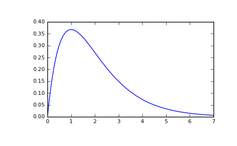
Second order system with a repeated root: x’‘(t) + 2*x(t) + x(t) = u(t)

>>> import scipy.signal
>>> system = ([1.0], [1.0, 2.0, 1.0])
>>> t, y = sp.signal.impulse2(system)
>>> import matplotlib.pyplot as plt
>>> plt.plot(t, y)

(Source code)